Polynomial Bases and Transformations#

Up until now, you’ve encountered Minterpy polynomials represented in the Lagrange and Newton bases. Minterpy supports a range of polynomial bases, all of which share a consistent interface. This means that regardless of the basis, polynomials can be manipulated and behave in a similar manner, making it easy to switch between different representations.

In this in-depth tutorial, you’ll explore:

Various polynomial bases supported by Minterpy;
Transformation between those bases.

For simplicity, this tutorial uses examples in one and two dimensions, but the principles apply to polynomials of higher dimensions as well.

Before diving in, make sure to import the necessary packages:

import minterpy as mp
import numpy as np
import matplotlib.pyplot as plt

import warnings
warnings.filterwarnings('ignore')

Polynomials in Minterpy#

Polynomials in Minterpy are multivariate polynomials defined on \([-1, 1]^m\) where \(m\) is the spatial dimension:

\[ Q(\boldsymbol{x}) = \sum_{\boldsymbol{\alpha} \in A} c_{\cdot, \boldsymbol{\alpha}} \Psi_{\cdot, \boldsymbol{\alpha}} (\boldsymbol{x}), \]

where:

\(A\) is the multi-index set of the exponents, i.e., \(\boldsymbol{\alpha} \in A \subseteq \mathbb{N}^m\) which generalizes the notion of polynomial degree to multiple dimensions.
\(\Psi_{\cdot, \boldsymbol{\alpha}}\) is the multidimensional basis polynomial associated with the multi-index element \(\boldsymbol{\alpha}\), the placeholder \(\cdot\) indicates that the basis polynomials depend on the chosen basis.
\(c_{\cdot, \boldsymbol{\alpha}}\) is the coefficient that corresponds to the multidimensional basis polynomial \(\Psi_{\cdot, \boldsymbol{\alpha}}\).

Minterpy supports several polynomial bases as shown in the table below.

Basis	Constructor
Lagrange	`LagrangePolynomial`
Newton	`NewtonPolynomial`
Canonical	`CanonicalPolynomial`
Chebyshev (of the 1st kind)	`ChebyshevPolynomial`

Lagrange basis#

The Lagrange basis was the first polynomial basis you encountered in this series of tutorials. In Minterpy, the multivariate Lagrange basis polynomial associated with the multi-index element \(\boldsymbol{\alpha}\) is defined as a polynomial that satisfies the following condition:

\[ \Psi_{\mathrm{lag}, \boldsymbol{\alpha}} (\boldsymbol{p}_{\boldsymbol{\beta}}) = \delta_{\boldsymbol{\alpha}, \boldsymbol{\beta}}, \;\; \boldsymbol{p}_{\boldsymbol{\beta}} \in P_{A}, \;\; \boldsymbol{\alpha}, \boldsymbol{\beta} \in A, \]

where \(P_{A}\) is the set of unisolvent nodes, \(A\) is the multi-index set of exponents, and \(\delta_{\cdot, \cdot}\) is the Kronecker delta.

Note

The condition above is necessary for defining the Lagrange basis polynomials, but it does not provide the full expression of these basis polynomials as functions of \(\boldsymbol{x} \in [-1, 1]^m\). Indeed in Minterpy, Lagrange basis polynomials are conceptual basis polynomials that can only be expressed in terms of another polynomial basis.

Polynomials in the Lagrange basis in Minterpy have limited functionality; for instance, they cannot be directly evaluated at a set of query points. Nevertheless, they serve as an entry point for function approximations using interpolating polynomials because their coefficients are highly intuitive. Specifically, the coefficient corresponding to the multi-index element \(\boldsymbol{\alpha}\) of an interpolating polynomial approximating a function \(f\) is

\[ c_{\mathrm{lag}, \boldsymbol{\alpha}} = f(\boldsymbol{p}_{\boldsymbol{\alpha}}), \;\; \boldsymbol{p}_{\boldsymbol{\alpha}} \in P_{A}, \;\; \boldsymbol{\alpha} \in A, \]

In other words, the coefficients are simply the values of the function at the unisolvent nodes.

To do more with the polynomials, such as evaluation or manipulation, you need to transform them to another basis. This process will be covered in a later section of this tutorial.

Newton basis#

You’ve also seen the Newton basis by following these tutorials. The multivariate Newton basis polynomial associated with multi-index element \(\alpha\) is defined as:

\[ \Psi_{\mathrm{nwt}, \boldsymbol{\alpha}} (\boldsymbol{x}) = \prod_{j = 1}^m \prod_{i = 0}^{\alpha_j - 1} (x_j - p_{i, j}), \]

where \(p_{i, j}\)’s are the interpolation points along dimension \(j\) (i.e., the so-called generating points / nodes which in multiple dimensions are not the same as the unisolvent nodes).

Note

As you can see in the above definition, the Newton basis polynomials depend on the generating points of an interpolation grid. Such points are an integral part of the definition of the basis.

As an example, consider the two-dimensional multi-index set:

\[ A = \{ (0, 0), (1, 0), (2, 0), (3, 0), (0, 1), (1, 1), (2, 1), (0, 2) \}. \]

Newton basis polynomial can only be defined with respect to a given generating points. Valid generating points that are distributed according to the Leja-ordered Chebyshev-Lobatto points are given in the table below.

\(\mathrm{dim} = 1\)	\(\mathrm{dim} = 2\)
\(1.0\)	\(-1.0\)
\(-1.0\)	\(1.0\)
\(0.5\)	\(-0.5\)

The Newton basis polynomials according to the above multi-index set of exponents are given in the table below.

\(\boldsymbol{\alpha} \in A\)	\(\Psi_{\mathrm{nwt}, \boldsymbol{\alpha} }\)
\((0, 0)\)	\(1.0\)
\((1, 0)\)	\(x_1 - 1.0\)
\((2, 0)\)	\((x_1 - 1.0) (x_1 + 1.0)\)
\((3, 0)\)	\((x_1 - 1.0) (x_1 + 1.0) (x_1 - 0.5)\)
\((0, 1)\)	\(x_2 + 1.0\)
\((1, 1)\)	\((x_1 - 1.0) (x_2 + 1.0)\)
\((2, 1)\)	\((x_1 - 1.0) (x_1 + 1.0) (x_2 + 1.0)\)
\((0, 2)\)	\((x_2 + 1.0) (x_2 - 1.0)\)

Canonical basis#

The canonical basis is arguably the most familiar polynomial basis of them all. The multivariate canonical basis polynomial associated with the multi-index element \(\boldsymbol{\alpha}\) is defined as:

\[ \Psi_{\mathrm{can}, \boldsymbol{\alpha}} (\boldsymbol{x}) = x_1^{\alpha_1} \cdots x_m^{\alpha_m} = \prod_{j = 1}^m x_j^{\alpha_j}. \]

Warning

Although polynomials in the canonical basis can be evaluated at a set of query points, it’s essential to note that high-degree polynomials in the canonical basis can become numerically unstable when evaluated. As a result, we strongly advise against using the canonical basis for high-degree polynomials due to potential numerical issues.

As an example, consider the two-dimensional multi-index set:

\[ A = \{ (0, 0) , (1, 0), (2, 0), (0, 1), (1, 1), (2, 1) \}. \]

The canonical basis polynomials according to the above multi-index set of exponents are given in the table below.

\(\boldsymbol{\alpha} \in A\)	\(\Psi_{\mathrm{can}, \boldsymbol{\alpha} }\)
\((0, 0)\)	\(1.0\)
\((1, 0)\)	\(x_1\)
\((2, 0)\)	\(x_1^2\)
\((0, 1)\)	\(x_2\)
\((1, 1)\)	\(x_1 x_2\)
\((2, 1)\)	\(x_1^2 x_2\)

Chebyshev basis#

The multivariate Chebyshev basis polynomial (of the first kind) associated with the multi-index element \(\boldsymbol{\alpha}\) is defined as:

\[ \Psi_{\mathrm{cheb}, \boldsymbol{\alpha}} (\boldsymbol{x}) = T_{\alpha_1} (x_1) \cdots T_{\alpha_m} (x_m) = \prod_{j = 1}^m T_{\alpha_j} (x_j), \]

where \(T_{\alpha_j} (x_j)\) is the \(\alpha_j\)th-degree univariate Chebyshev polynomial of the first kind associated with the \(j\)th-dimension.

The univariate Chebyshev polynomial of the first kind satisfies the following three-term recurrence (TTR) relation:

\[\begin{split} \begin{aligned} T_0 (x) & = 1 \\ T_1 (x) & = x \\ T_{n + 1} (x) & = 2 \, x \, T_n(x) - T_{n - 1} (x) \end{aligned} \end{split}\]

As an example, consider the two-dimensional multi-index set:

\[ A = \{ (0, 0) , (1, 0), (2, 0), (0, 1), (1, 1) \}. \]

The Chebyshev basis polynomial (of the first kind) according to the above multi-index set of exponents are given in the table below.

\(\boldsymbol{\alpha} \in A\)	\(\Psi_{\mathrm{cheb}, \boldsymbol{\alpha}}\)	Full expression
\((0, 0)\)	\(T_0 (x_1) T_0 (x_2)\)	\(1.0\)
\((1, 0)\)	\(T_1 (x_1) T_0 (x_2)\)	\(x_1\)
\((2, 0)\)	\(T_2 (x_1) T_0 (x_2)\)	\(2 x_1^2 - 1\)
\((0, 1)\)	\(T_0 (x_1) T_1 (x_2)\)	\(x_2\)
\((1, 1)\)	\(T_1 (x_1) T_1 (x_2)\)	\(x_1 x_2\)

Change of basis#

Polynomials represented in one basis can be transformed into a polynomial in another basis with the help of various transformation classes listed in the tables below.

From Lagrange To…	Transformation
Newton	`LagrangeToNewton`
Canonical	`LagrangeToCanonical`
Chebyshev	`LagrangeToChebyshev`
From Newton To…
Lagrange	`NewtonToLagrange`
Canonical	`NewtonToCanonical`
Chebyshev	`NewtonToChebyshev`
From canonical To…
Lagrange	`CanonicalToLagrange`
Newton	`CanonicalToNewton`
Chebyshev	`CanonicalToChebyshev`
From Chebyshev To…
Lagrange	`ChebyshevToLagrange`
Newton	`ChebyshevToNewton`
Canonical	`ChebyshevToCanonical`

For demonstrantion, see a couple of examples below.

Example: One-dimensional polynomial#

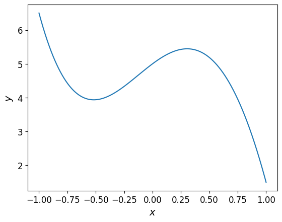
Consider the following one-dimensional polynomial:

\[ Q(x) = 5 + 2.5 x - 2.0 x^2 - 5.0 x^3 + 1.0 x^4, x \in [-1, 1]. \]

This polynomial is readily expressed in the canonical basis.

First, create the multi-index set of the polynomial:

mi_1d = mp.MultiIndexSet(np.array([[0], [1], [2], [3], [4]]), lp_degree=1.0)

Then store the coefficients in an array with the order that corresponds to the above multi-index set:

coeffs_1d = np.array([5., 2.5, -2., -5., 1.])

Finally, construct a polynomial in the canonical basis:

can_poly_1d = mp.CanonicalPolynomial(mi_1d, coeffs_1d)
can_poly_1d

<minterpy.polynomials.canonical_polynomial.CanonicalPolynomial at 0x7f0462ebeb30>

The plot of the polynomial is shown below.

../_images/030fa32eafa672cc36f5a6889ee3db779ac76440b0c575c37666c204a6081c5e.png

The same polynomial can be expressed in a different basis using the help of a transformation class. Note that all instance of the transformation class must be called to carry out the actual transformation that returns a polynomial in the new basis.

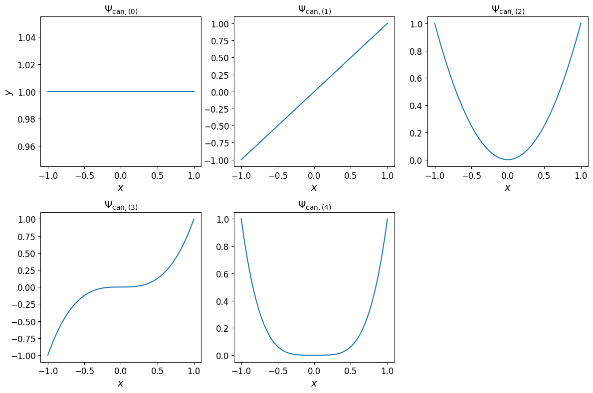
The univariate canonical basis polynomial are shown in the plots below.

../_images/ab62be31f5cff195ad39b207386112881f2a85d0957f23e20bbc0fe319ca0a0f.png

In the (1D) Lagrange basis#

The transformation of a polynomial in the canonical basis to the one in the Lagrange basis is carried out by an instance of CanonicalToLagrange:

lag_poly_1d = mp.CanonicalToLagrange(can_poly_1d)()

The coefficients of the Lagrange polynomial are:

lag_poly_1d.coeffs

array([1.5 , 6.5 , 5.  , 4.25, 4.25])

These coefficients are the function values at the unisolvent nodes:

can_poly_1d(can_poly_1d.grid.unisolvent_nodes)

array([1.5 , 6.5 , 5.  , 4.25, 4.25])

Note

Although the canonical polynomial can be defined without the need for an interpolation grid, the transformation to a Lagrange basis requires such a grid. If not specified during construction, Minterpy automatically creates an interpolating grid based on the Leja-ordered Chebyshev-Lobatto points.

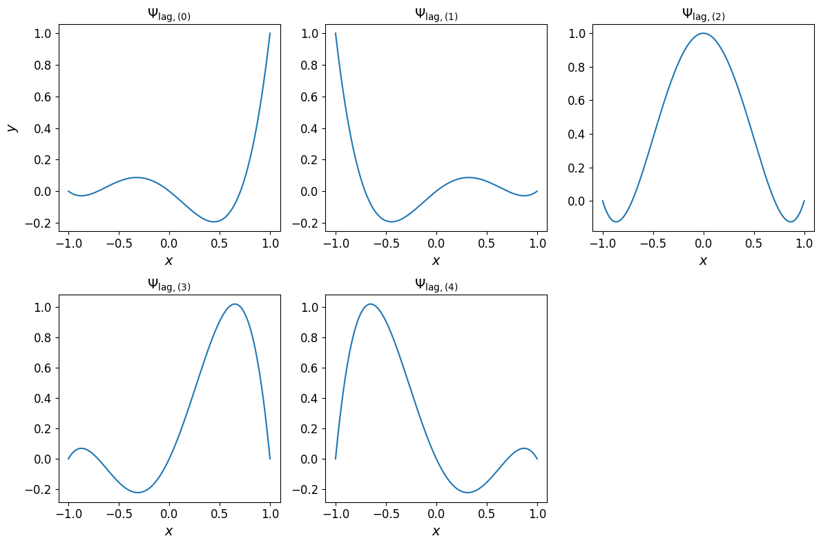
The one-dimensional Lagrange basis polynomials are shown in the plots below.

../_images/8e85af43789bdf6757019f367caf15a7f43d6c749bbc593fb2ecb8ba7d068a2b.png

In the (1D) Newton basis#

The transformation of a polynomial in the canonical basis to the one in the Newton basis is carried out by an instance of CanonicalToNewton:

nwt_poly_1d = mp.CanonicalToNewton(can_poly_1d)()

The coefficients of the Newton polynomial are:

nwt_poly_1d.coeffs

array([ 1.5       , -2.5       , -1.        , -4.29289322,  1.        ])

Although the canonical polynomial can be defined without the need for an interpolation grid, the transformation to a Newton basis requires such a grid. If not specified during construction, Minterpy automatically creates an interpolating grid based on the Leja-ordered Chebyshev-Lobatto points. This means the generating points of the grid are:

nwt_poly_1d.grid.generating_points

array([[ 1.00000000e+00],
       [-1.00000000e+00],
       [-6.12323400e-17],
       [ 7.07106781e-01],
       [-7.07106781e-01]])

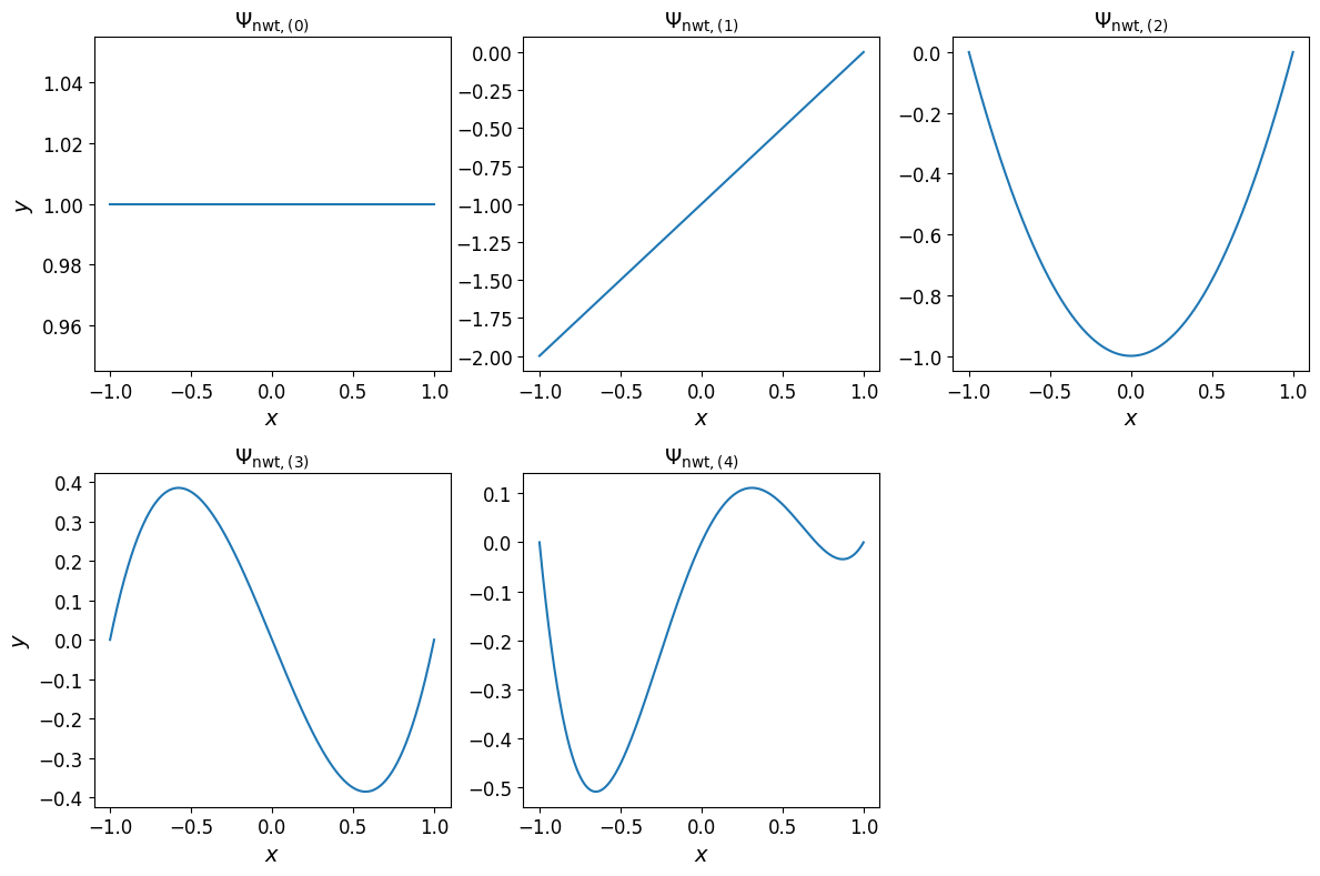
With these coefficients and generating points, the same polynomial can be expressed in the Newton basis as follows:

\[ Q(x) = 1.5 - 2.5 (x - 1) - 1 (x - 1) (x + 1) - 4.29289322 (x - 1) (x + 1) x + (x - 1) (x + 1) x (x - 0.707106781). \]

The one-dimensional Newton basis polynomials are shown in the plots below.

../_images/c2e7f3d709c1adfac134bbdc3e2cfcbb4d5a2afeaafdea64ad9bac4930c964ff.png

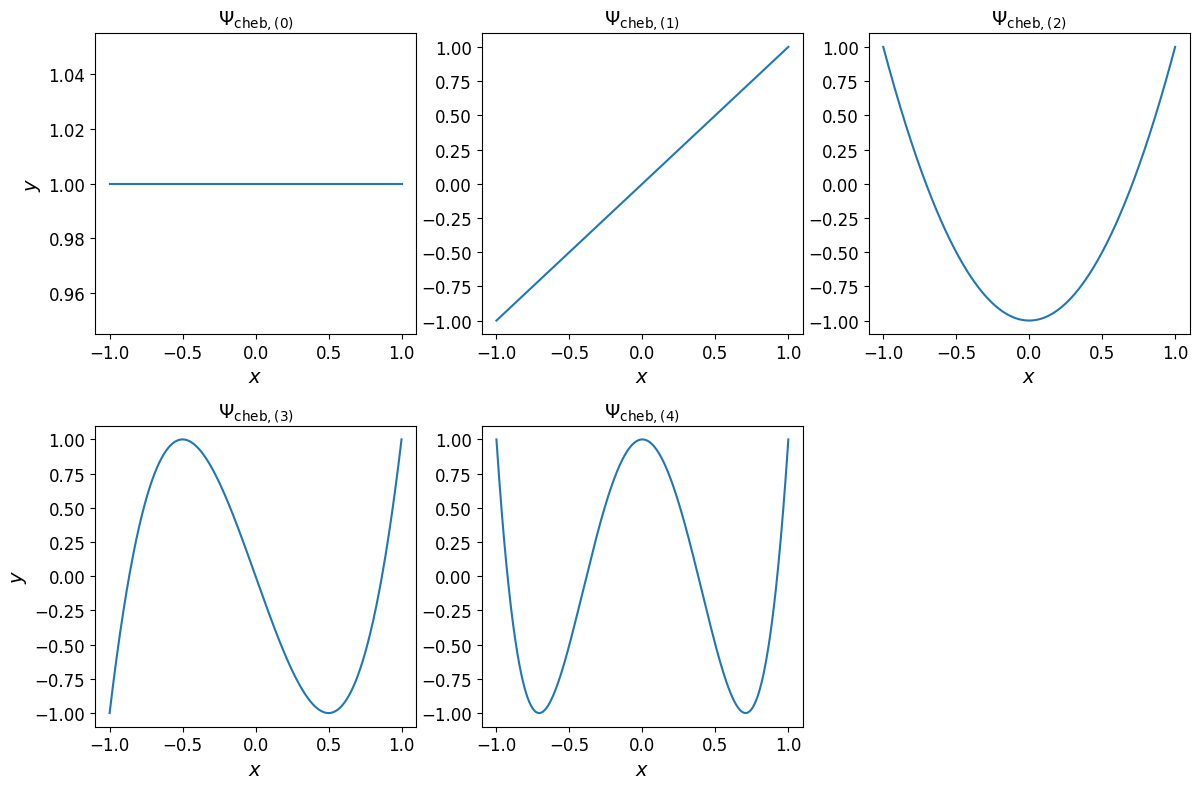
In the (1D) Chebyshev basis#

The transformation of a polynomial in the canonical basis to the one in the Chebyshev basis is carried out by an instance of CanonicalToChebyshev:

cheb_poly_1d = mp.CanonicalToChebyshev(can_poly_1d)()

The coefficients of the Chebyshev polynomial are:

cheb_poly_1d.coeffs

array([ 4.375, -1.25 , -0.5  , -1.25 ,  0.125])

With these coefficients and generating points, the same polynomial can be expressed in the Chebyshev basis as follows:

\[ Q(x) = 4.375 - 1.25 T_1 (x) - 0.5 T_2 (x) - 1.25 T_3 (x) + 0.125 T_4(x). \]

The one-dimensional Chebyshev basis polynomials are shown in the plots below.

../_images/8c7d5995ae11de8851119ec6422f1ee61e8586ad1a5d298a38c13f89f9fd2b55.png

Example: Two-dimensional polynomial#

Consider now the two-dimensional function:

\[ f(x_1, x_2) = \left( 25 - (x_1 - 0.5)^2 - (x_2 - 0.5)^2 \right)^{0.5}, x_1, x_2 \in [-1, 1]. \]

The function is defined in Python as follows:

def fun(xx):
    return np.sqrt(25 - (xx[:, 0] - 0.5)**2 - (xx[:, 1] - 0.5)**2)

../_images/c5166f2581821661f042ca1a0c9b7392e9c2d008d60244da537ebbc8659936b6.png

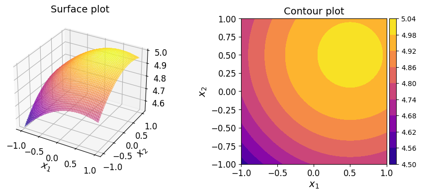
Since the function involves a square root and therefore is not a polynomial, constructing a polynomial approximation is much more intuitive in the Lagrange basis. In contrast, it’s not immediately clear what the coefficient values should be in other bases, making the Lagrange basis a more natural choce for this type of approximation.

First, create a two-dimensional multi-index with the following choices of \(n\) and \(p\):

mi_2d = mp.MultiIndexSet.from_degree(2, 3, 1.0)
mi_2d

MultiIndexSet(
  array([[0, 0],
         [1, 0],
         [2, 0],
         [3, 0],
         [0, 1],
         [1, 1],
         [2, 1],
         [0, 2],
         [1, 2],
         [0, 3]]),
  lp_degree=1.0
)

Then, create an interpolation grid and evaluate the function at the unisolvent nodes:

# Interpolation grid
grd_2d = mp.Grid(mi_2d)
# Coefficients of the Lagrange polynomial
lag_coeffs_2d = grd_2d(fun)

Finally, construct a polynomial in the Lagrange basis given the grid and coefficients:

lag_poly_2d = mp.LagrangePolynomial.from_grid(grd_2d, lag_coeffs_2d)

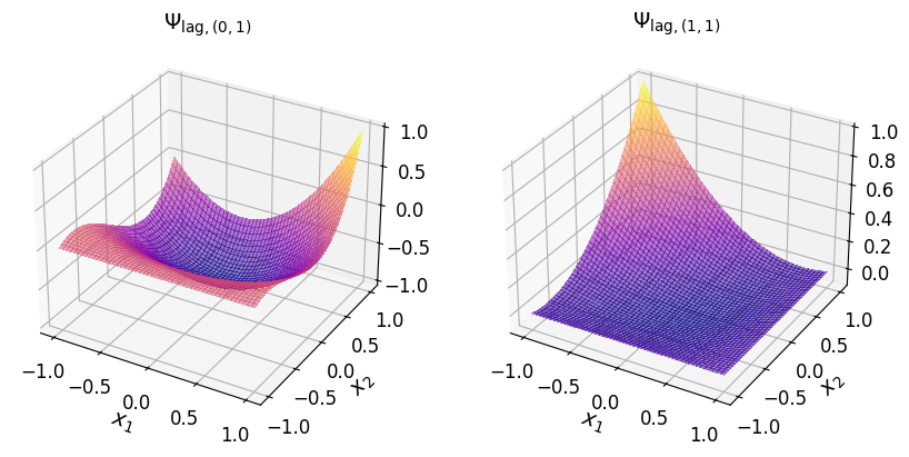
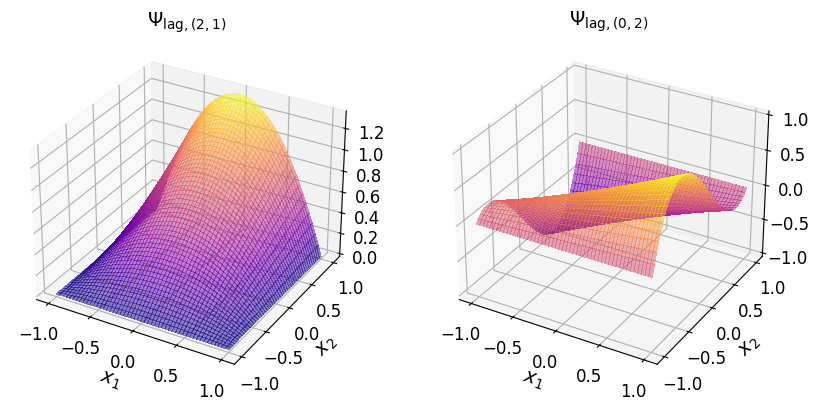
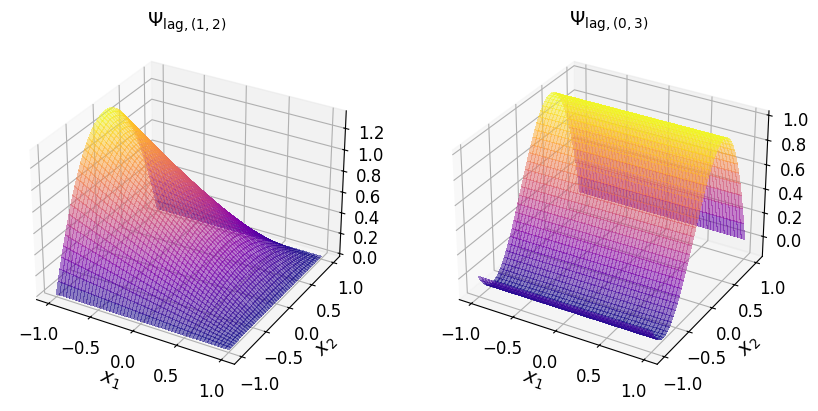
The two-dimensional Lagrange basis polynomials are shown in the plots below.

../_images/271f31911269dee218b715f262f9a26ab87dfe59492cfa5840e1c6c7455ed716.png

../_images/3024a6c0a14346de26bf7c24084c0101be926abe91694a2d0e2a5a0ef69cdff1.png

../_images/b403d7f56ec3da0d5b22777376b31634746882b93aeae2b01eee8bf40f627e6b.png

../_images/7c2fef60d525d8e1108bd075ad74da888725ad0fc91ac7206e431d00a93d8f77.png

../_images/a29fa88e14a3c415d3875f8dc90ab4e7dec99301c11aa59b4ba554fe4574eca1.png

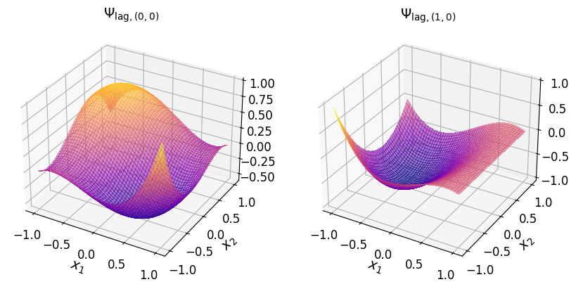
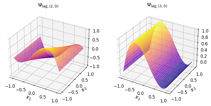
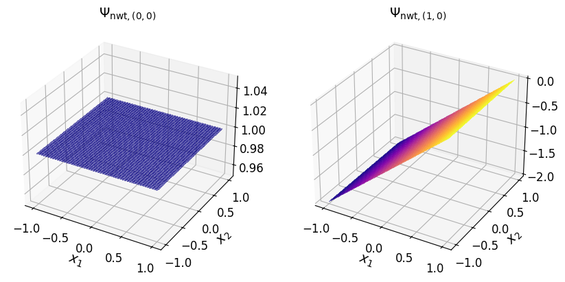
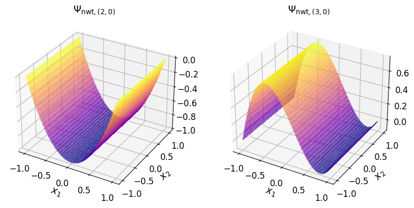
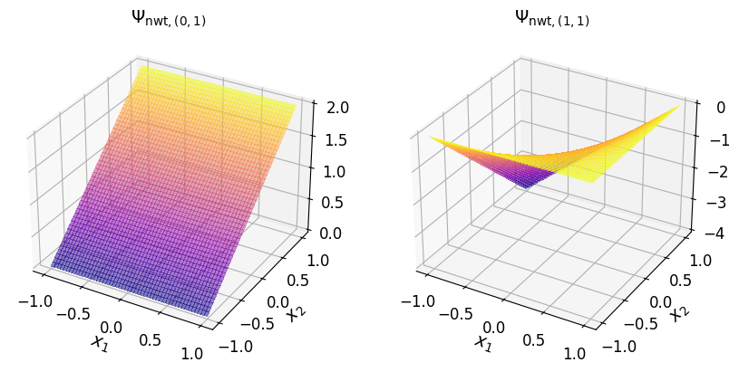
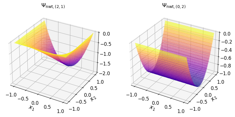
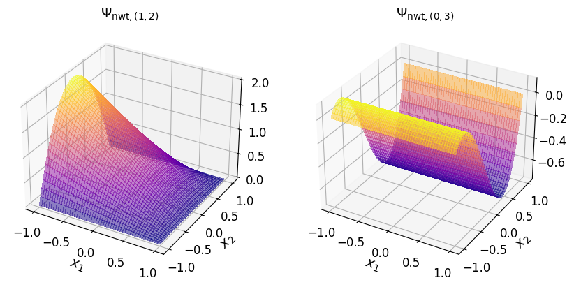
In the (2D) Newton basis#

You can transform a Minterpy polynomial in the Lagrange basis to another polynomial in the Newton basis with the help of LagrangeToNewton:

nwt_poly_2d = mp.LagrangeToNewton(lag_poly_2d)()

The coefficients of the Newton polynomial are:

nwt_poly_2d.coeffs

array([ 4.74341649e+00,  1.07861961e-01, -1.06947330e-01,  2.47397340e-03,
        1.03165489e-01, -2.34823578e-03,  2.29202359e-03, -1.04530584e-01,
        2.44535969e-03,  2.16730120e-03])

The two-dimensional Newton basis polynomials are shown in the plots below.

../_images/a9a696c028bc1763eb14afea18dfa2efee00429894e93d87e0c104a053e5c5f5.png

../_images/88686bba2c3616cb03aa2ce8501c78e1d2e94688ee8db7429b387ba403f107f6.png

../_images/5a23e704ce7d54c20d118961424f78b641c314d2b6be286c0791f6aee0efe2ad.png

../_images/a6465c2211f5814f36ea1e12954ccb0aed8e1ab53352070d9fefe1fdbfd0d056.png

../_images/874e566cdd40632dfcfd356fee254db1450b1559c0f8a424d4c86f8eeb369521.png

In the (2D) canonical basis#

You can transform a Minterpy polynomial in the Lagrange basis to another polynomial in the canonical basis with the help of LagrangeToCanonical:

can_poly_2d = mp.LagrangeToCanonical(lag_poly_2d)()

The coefficients of the canonical polynomial are:

can_poly_2d.coeffs

array([ 4.95285284e+00,  1.00594392e-01, -1.05892293e-01,  2.47397340e-03,
        1.01054400e-01, -2.34823578e-03,  2.29202359e-03, -1.05892293e-01,
        2.44535969e-03,  2.16730120e-03])

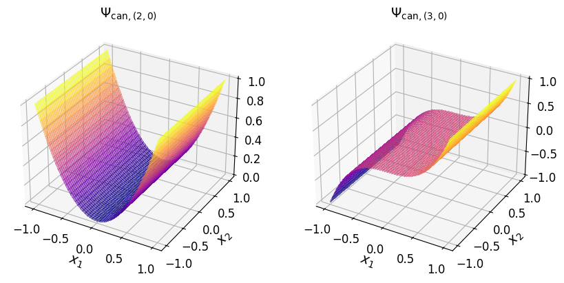
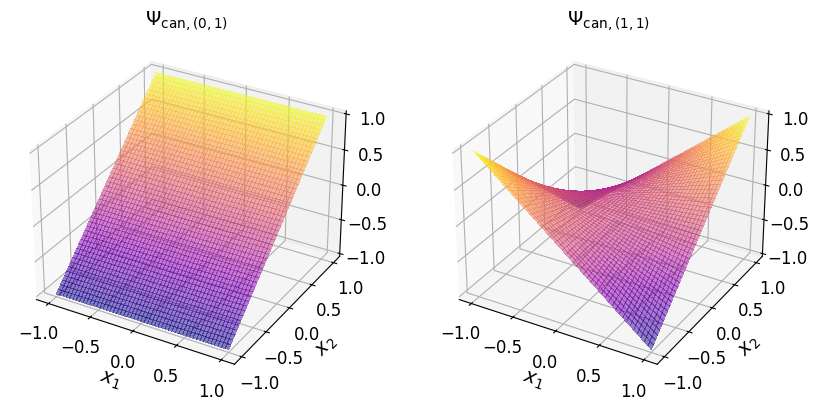
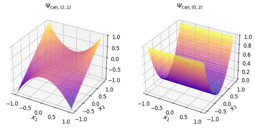
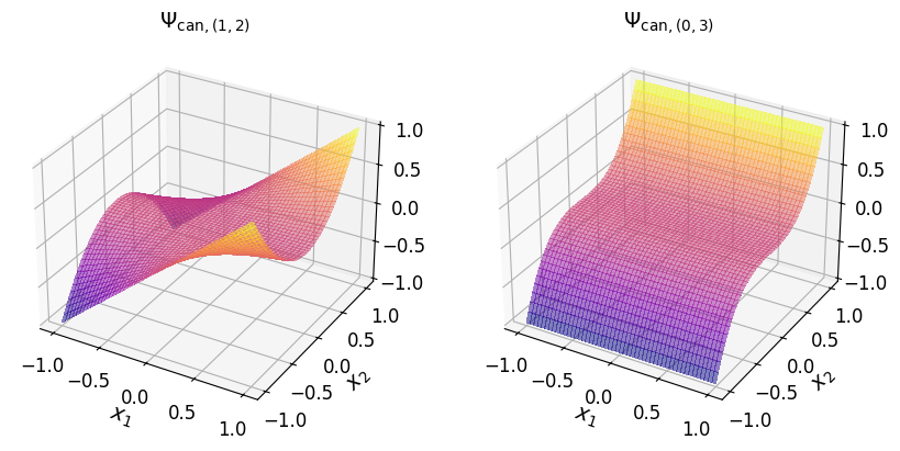
The two-dimensional canonical basis polynomials are shown in the plots below.

../_images/00cde596ff0b0e6a1f6b33659f1e1443f00fd850f13bdce869e52b39d5863a89.png

../_images/9d4e7c73a94f57b38f70cb5cd9b187841c3c5ac2894445a5993bdb869bc06a69.png

../_images/c56e11ead5c4b0e09845fd79eac0047945d8baf7ffa01722c5a82329ca1b430b.png

../_images/9a8591ce4731d6d36d213b5421a539132c07fa01c25c6ab1f99527b845afda45.png

../_images/42bdb95d5b31a80dd4500104ca241e161907cef1e52696faf7e99da41f3f1e90.png

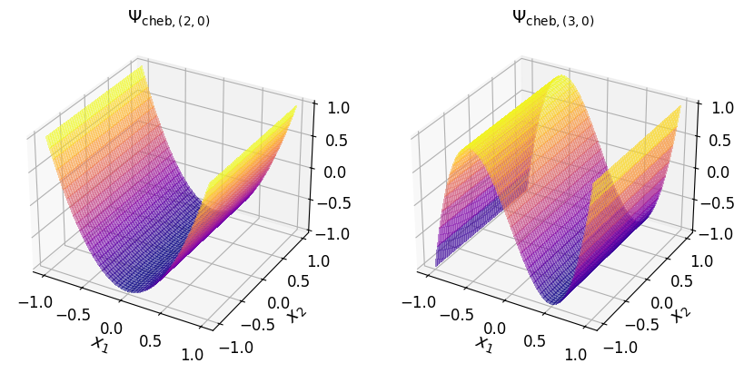
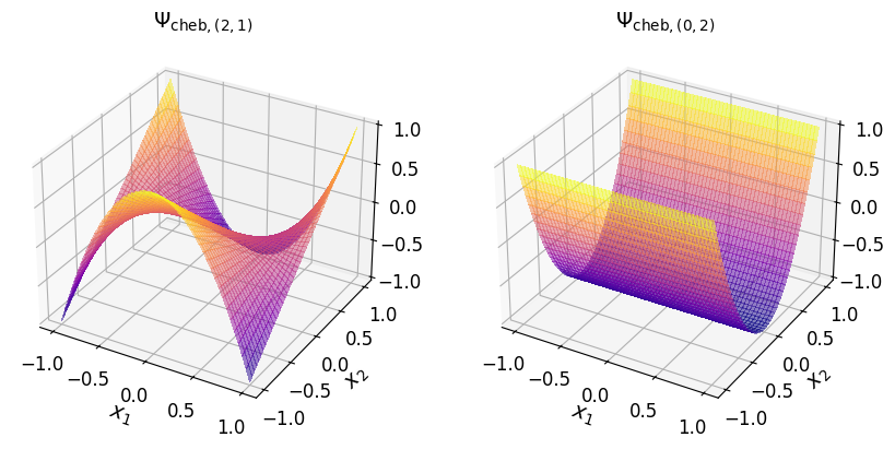
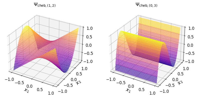
In the (2D) Chebyshev basis#

Finally, you can transform a Minterpy polynomial in the Lagrange basis to another polynomial in the Chebyshev basis (of the first kind) with the help of LagrangeToChebyshev:

cheb_poly_2d = mp.LagrangeToChebyshev(lag_poly_2d)()

The coefficients of the canonical polynomial are:

cheb_poly_2d.coeffs

array([ 4.84696055e+00,  1.03672552e-01, -5.29461463e-02,  6.18493351e-04,
        1.03825888e-01, -2.34823578e-03,  1.14601180e-03, -5.29461463e-02,
        1.22267985e-03,  5.41825299e-04])

The two-dimensional Chebyshev basis polynomials (of the first kind) are shown in the plots below.

../_images/120a69de43e06b592d668ff59152e4ad975f3796459c7823f71763bf0929d771.png

../_images/0d6e045147ff3cc2c81d867fc0123c5ef95cf22462ecb460f6de16ff6b44f069.png

../_images/437d6255fd5f2cc56af6290b9b8824873ca3c04a28a35598a76981bd9407a2b8.png

../_images/1ae1e7ce4adcb9282da562daa6262b944212c574bd155de16c36347c8a0c0748.png

../_images/2f03054e5922ba83b8148cbe817e399ead7e99fab885f2fb8662157f5b88aded.png

From interpolant to interpolating polynomial#

The Quickstart Guide introduced you with the interpolate() function to conveniently create an interpolant out of a function for a given spatial dimension, polynomial degree, and \(l_p\)-degree. As noted in the previous tutorials, while interpolate() does not produce an instance of Minterpy polynomials (and instead, an instance of Interpolant) you can conveniently retrieve the polynomial by the methods summarized in the table below.

Method	Return the interpolant as a polynomial in the…
`to_newton()`	`NewtonPolynomial`
`to_lagrange()`	`LagrangePolynomial`
`to_canonical()`	`CanonicalPolynomial`
`to_chebyshev()`	`CanonicalPolynomial`

Summary#

In this tutorial, you’ve explored the different polynomial bases supported by Minterpy. Depending on the problem at hand, it may be more intuitive to construct a polynomial in a specific basis.

One of the powerful features of Minterpy is the ability to transform a polynomial from one basis to another. This transformation produces a new polynomial that is mathematically equivalent to the original, but expressed in a different basis.

Keep in mind that Minterpy’s supported features vary across different polynomial bases. The following table provides a summary of the available features for each basis.

Operations	Lagrange	Newton	Canonical	Chebyshev
Transformation from-and-to	✓	✓	✓	✓
Evaluation	✕	✓	✓	✓
Addition/Subtraction (Scalar)	✓	✓	✓	✓
Addition/Subtraction (Polynomial)	✕	✓	✓	✓
Multiplication (Scalar)	✓	✓	✓	✓
Multiplication (Polynomial)	✕	✓	✓	✓
Division (Scalar)	✓	✓	✓	✓
Division (Polynomial)	✕	✕	✕	✕
Differentiation	✕	✓	✓	✕
Definite integration	✕	✓	✓	✕

To recap, you’ve now acquired a solid foundation in working with Minterpy polynomials, including:

Constructing polynomials in one or more dimensions;
Performing various operations with polynomials, such as arithmetic and calculus operations;
Understanding the different polynomial bases and transforming between them (this tutorial).

In all these tutorials, you typically start with a given function of interest, where you can evaluate it at specifically chosen locations (i.e., the unisolvent nodes) to construct an interpolating polynomial.

One important problem remains: How do you construct a polynomial from a given set of scattered data?