Basic Calculus Operations with Polynomials

So far, you’ve learned how to construct interpolating polynomials in both one and multiple dimensions. You’ve also explored the basic arithmetic operations supported by Minterpy polynomials.

In this in-depth tutorial, you’ll learn about the basic calculus operations that can be performed with Minterpy polynomials.

As usual, before you begin, you’ll need to import the necessary packages to follow along with this guide.

import minterpy as mp
import numpy as np
import matplotlib.pyplot as plt

Motivating function

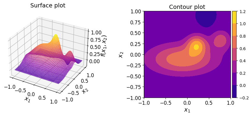
Consider the following two-dimensional function:

\[\begin{split} \begin{align} \mathcal{M}(\boldsymbol{x}) = & 0.75 \exp{\left( -0.25 \left( (x_1 - 2)^2 + (x_2 - 2)^2 \right) \right) } \\ & + 0.75 \exp{\left( -1.00 \left( \frac{(x_1 + 1)^2}{49} + \frac{(x_2 + 1)^2}{10} \right) \right)} \\ & + 0.50 \exp{\left( -0.25 \left( (x_1 - 7)^2 + (x_2 - 3)^2 \right) \right)} \\ & - 0.20 \exp{\left( -1.00 \left( (x_1 - 4)^2 + (x_2 - 7)^2 \right) \right)} \\ \end{align} \end{split}\]

where \(\boldsymbol{x} = (x_1, x_2) \in [-1, 1]^2\).

Note

This function is known in the literature as the Franke function[1]. Here, however, the domain has been redefined to be \([-1, 1]^2\) instead of \([0, 1]^2\).

The function can be defined in Python as follows:

def fun(xx: np.ndarray):
    xx0 = 9 * xx[:, 0]
    xx1 = 9 * xx[:, 1]

    # Compute the (first) Franke function
    term_1 = 0.75 * np.exp(-0.25 * ((xx0 - 2) ** 2 + (xx1 - 2) ** 2))
    term_2 = 0.75 * np.exp(
        -1.00 * ((xx0 + 1) ** 2 / 49.0 + (xx1 + 1) ** 2 / 10.0)
    )
    term_3 = 0.50 * np.exp(-0.25 * ((xx0 - 7) ** 2 + (xx1 - 3) ** 2))
    term_4 = 0.20 * np.exp(-1.00 * ((xx0 - 4) ** 2 + (xx1 - 7) ** 2))

    yy = term_1 + term_2 + term_3 - term_4

    return yy

The surface and contour plots of the function are shown below.

Show code cell source Hide code cell source

from mpl_toolkits.axes_grid1 import make_axes_locatable

# --- Create 2D data
xx_1d = np.linspace(-1.0, 1.0, 500)[:, np.newaxis]
mesh_2d = np.meshgrid(xx_1d, xx_1d)
xx_2d = np.array(mesh_2d).T.reshape(-1, 2)
yy_2d = fun(xx_2d)

# --- Create two-dimensional plots
fig = plt.figure(figsize=(10, 5))

# Surface
axs_1 = plt.subplot(121, projection='3d')
axs_1.plot_surface(
    mesh_2d[0],
    mesh_2d[1],
    yy_2d.reshape(500, 500).T,
    linewidth=0,
    cmap="plasma",
    antialiased=False,
    alpha=0.5
)
axs_1.set_xlabel("$x_1$", fontsize=14)
axs_1.set_ylabel("$x_2$", fontsize=14)
axs_1.set_zlabel("$f(x_1, x_2)$", fontsize=14)
axs_1.set_title("Surface plot", fontsize=14)
axs_1.tick_params(axis='both', which='major', labelsize=12)

# Contour
axs_2 = plt.subplot(122)
cf = axs_2.contourf(
    mesh_2d[0], mesh_2d[1], yy_2d.reshape(500, 500).T, cmap="plasma"
)
axs_2.set_xlabel("$x_1$", fontsize=14)
axs_2.set_ylabel("$x_2$", fontsize=14)
axs_2.set_title("Contour plot", fontsize=14)
divider = make_axes_locatable(axs_2)
cax = divider.append_axes('right', size='5%', pad=0.05)
fig.colorbar(cf, cax=cax, orientation='vertical')
axs_2.axis('scaled')
axs_2.tick_params(axis='both', which='major', labelsize=12)

fig.tight_layout(pad=6.0)

You can construct a (Newton) polynomial that approximates the above function with the following:

# Multi-index set of polynomial degree
mi = mp.MultiIndexSet.from_degree(2, 75, 1.0)
# Interpolation grid
grd = mp.Grid(mi)
# Coefficients of the Lagrange polynomial
coeffs = grd(fun)
# Lagrange polynomial given grid and coefficients
lag_poly = mp.LagrangePolynomial.from_grid(grd, coeffs)
# Transformation to the Newton basis
poly = mp.LagrangeToNewton(lag_poly)()                 

Verify if the interpolating polynomial has the sufficient accuracy by estimating its infinity norm:

xx_test = -1 + 2 * np.random.rand(10000, 2)
yy_test = fun(xx_test)
yy_poly = poly(xx_test)
print(np.max(np.abs(yy_poly - yy_test)))

6.171521084561045e-07

Integration

Minterpy polynomials support definite integration via the method integrate_over().

Specifically, calling the method on a polynomial computes the following expression:

\[ I[Q] = \int_{\Omega} Q(\boldsymbol{x}) \, d\boldsymbol{x}, \]

where \(\Omega\) is the domain of the polynomial which in this case is \([-1, 1]^2\).

poly.integrate_over()

0.7757899777014259

Note

Instances of most polynomial bases in Minterpy support the method integrate_over(); if the method is not yet implemented for a particular basis then an exception will be raised.

To define custom bounds for definite integration in Minterpy, pass a list of lists, where each inner list specifies the lower and upper bounds for a particular dimension, in the order dimension (i.e., the first inner list corresponds to the first dimension, the second inner list corresponds to the second dimension, and so on). This enables you to compute integrals over specific regions of interest.

For instance, to compute:

\[ \int_{-0.5}^{0.5} \int_{-0.25}^{0.75} Q(\boldsymbol{x}) \, dx_2 dx_1, \]

you would specify the bounds for each dimension as follows:

poly.integrate_over(bounds=[[-0.5, 0.5], [-0.25, 0.75]])

0.39984157731754727

Differentiation

Minterpy polynomials also supports differentiation via two methods:

• partial_diff()

• diff()

Note

Just like definite integration, instances of Minterpy polynomial bases may or may not support the methods; if the method is not yet implemented for a particular basis then an exception will be raised.

The method partial_diff() accepts two integer arguments: the spatial dimension specification and the order of derivative.

See the following table for examples.

Command	Expression
poly.partial_diff(0)	\(\frac{\partial Q}{\partial x_1}\)
poly.partial_diff(0, 1)	\(\frac{\partial Q}{\partial x_1}\)
poly.partial_diff(0, 2)	\(\frac{\partial^2 Q}{\partial x_1^2}\)
poly.partial_diff(1, 3)	\(\frac{\partial^3 Q}{\partial x_2^3}\)

The second argument is optional; if not specified then it will be set to \(1\) (i.e., first order of derivative).

Note

The spatial dimension specification starts with \(0\), i.e., \(0\) is the index for the first spatial dimension.

Calling partial_diff() on an instance of polynomial returns another instance of polynomial.

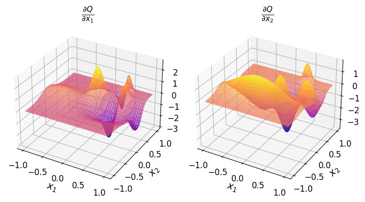
For instance, to obtain the polynomial \(\frac{\partial Q}{\partial x_1}\):

poly_diff_0_1 = poly.partial_diff(0)
poly_diff_0_1

<minterpy.polynomials.newton_polynomial.NewtonPolynomial at 0x7ff3658bc7f0>

or the polynomial \(\frac{\partial Q}{\partial x_2}\):

poly_diff_1_1 = poly.partial_diff(1)
poly_diff_1_1

<minterpy.polynomials.newton_polynomial.NewtonPolynomial at 0x7ff3658bfb20>

Show code cell source Hide code cell source

# --- Create 2D data
xx_1d = np.linspace(-1.0, 1.0, 500)[:, np.newaxis]
mesh_2d = np.meshgrid(xx_1d, xx_1d)
xx_2d = np.array(mesh_2d).T.reshape(-1, 2)
yy_diff_0_1 = poly_diff_0_1(xx_2d)
yy_diff_1_1 = poly_diff_1_1(xx_2d)

# --- Create two-dimensional plots
fig, axs = plt.subplots(
    nrows=1,
    ncols=2,
    figsize=(12, 4),
    subplot_kw=dict(projection="3d"),
    layout="compressed",
)

# Original function
axs[0].plot_surface(
    mesh_2d[0],
    mesh_2d[1],
    yy_diff_0_1.reshape(500, 500).T,
    linewidth=0,
    cmap="plasma",
    antialiased=False,
    alpha=0.5
)
axs[0].set_xlabel("$x_1$", fontsize=14)
axs[0].set_ylabel("$x_2$", fontsize=14)
axs[0].set_title("$\\frac{\\partial Q}{\\partial x_1}$", fontsize=16)
axs[0].tick_params(axis='both', which='major', labelsize=12)

# Interpolating polynomial
axs[1].plot_surface(
    mesh_2d[0],
    mesh_2d[1],
    yy_diff_1_1.reshape(500, 500).T,
    linewidth=0,
    cmap="plasma",
    antialiased=False,
    alpha=0.5
)
axs[1].set_xlabel("$x_1$", fontsize=14)
axs[1].set_ylabel("$x_2$", fontsize=14)
axs[1].set_title("$\\frac{\\partial Q}{\\partial x_2}$", fontsize=16)
axs[1].tick_params(axis='both', which='major', labelsize=12)

The diff() method enables you to compute the derivatives of varying oders for each spatial dimension simultaneously. To do this, pass a list or a NumPy array specifying the desired order of derivative for each dimension.

See the following table for examples.

Command	Expression
poly.diff([1, 1])	\(\frac{\partial^2 Q}{\partial x_1 \partial x_2}\)
poly.diff([0, 1])	\(\frac{\partial Q}{\partial x_2}\)
poly.diff([1, 2])	\(\frac{\partial^3 Q}{\partial x_1 \partial x_2^2}\)
poly.diff([3, 1])	\(\frac{\partial^4 Q}{\partial x_1^3 \partial x_2}\)

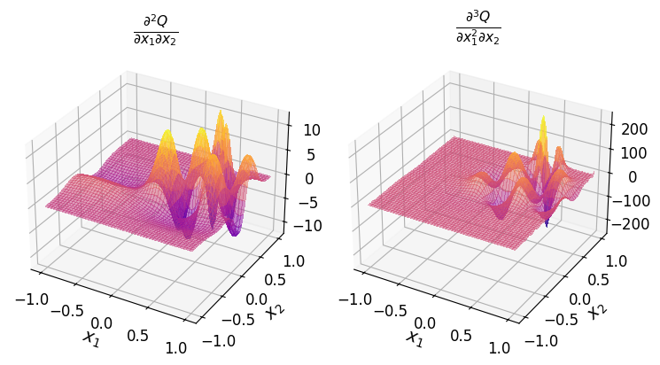
For instance, to obtain the polynomial \(\frac{\partial^2 Q}{\partial x_1 \partial x_2}\):

poly_diff_0_1_1_1 = poly.diff([1, 1])
poly_diff_0_1_1_1

<minterpy.polynomials.newton_polynomial.NewtonPolynomial at 0x7ff360781060>

or the polynomial \(\frac{\partial^3 Q}{\partial x_1^2 \partial x_2}\):

poly_diff_0_2_1_1 = poly.diff([2, 1])
poly_diff_0_2_1_1

<minterpy.polynomials.newton_polynomial.NewtonPolynomial at 0x7ff363d250f0>

Show code cell source Hide code cell source

# --- Create 2D data
xx_1d = np.linspace(-1.0, 1.0, 500)[:, np.newaxis]
mesh_2d = np.meshgrid(xx_1d, xx_1d)
xx_2d = np.array(mesh_2d).T.reshape(-1, 2)
yy_diff_0_1_1_1 = poly_diff_0_1_1_1(xx_2d)
yy_diff_0_2_1_1 = poly_diff_0_2_1_1(xx_2d)

# --- Create two-dimensional plots
fig, axs = plt.subplots(
    nrows=1,
    ncols=2,
    figsize=(12, 4),
    subplot_kw=dict(projection="3d"),
    layout="compressed",
)

# Original function
axs[0].plot_surface(
    mesh_2d[0],
    mesh_2d[1],
    yy_diff_0_1_1_1.reshape(500, 500).T,
    linewidth=0,
    cmap="plasma",
    antialiased=False,
    alpha=0.5
)
axs[0].set_xlabel("$x_1$", fontsize=14)
axs[0].set_ylabel("$x_2$", fontsize=14)
axs[0].set_title("$\\frac{\\partial^2 Q}{\\partial x_1 \\partial x_2}$", fontsize=16)
axs[0].tick_params(axis='both', which='major', labelsize=12)

# Interpolating polynomial
axs[1].plot_surface(
    mesh_2d[0],
    mesh_2d[1],
    yy_diff_0_2_1_1.reshape(500, 500).T,
    linewidth=0,
    cmap="plasma",
    antialiased=False,
    alpha=0.5
)
axs[1].set_xlabel("$x_1$", fontsize=14)
axs[1].set_ylabel("$x_2$", fontsize=14)
axs[1].set_title("$\\frac{\\partial^3 Q}{\\partial x_1^2 \\partial x_2}$", fontsize=16)
axs[1].tick_params(axis='both', which='major', labelsize=12)

Summary

In this in-depth tutorial, you’ve learned the basic calculus operations involving Minterpy polynomials, specifically:

• Definite integration: Computes the integral over specified bounds, returning a numeric result.

• Differentiation: Computes the derivative of the polynomial, resulting in another polynomial (the differentiated one).

These operations were demonstrated using a two-dimensional polynomial, but they apply similarly to polynomials of higher dimensions.

---

Throughout this series of in-depth tutorials, we’ve explored the following topics:

• Constructing Minterpy polynomials, from simple one-dimensional cases to more complex multivariate ones;

• Performing basic arithmetic operations with Minterpy polynomials, including addition, subtraction, and multiplication;

• Applying basic calculus operations to Minterpy polynomials, including differentiation and definite integration (this tutorial).

In the examples we’ve explored so far, we’ve started with a polynomial in the Lagrange basis and then converted it to a polynomial in the Newton basis. However, Minterpy offers more flexibility than that.

Polynomials can be represented in a variety of bases, extending beyond just Lagrange and Newton. In the next tutorial, we’ll delve into different bases available in Minterpy and discuss how to transform polynomials between the.

---

[1]

Richard Franke, “A critical comparison of some methods for interpolation of scattered data,” Naval Postgraduate School, Monterey, Canada, Technical Report No. NPS53-79-003, 1979. URL: https://core.ac.uk/reader/36727660