Multivariate Polynomial Interpolation#

In the previous guide, you learned the basics of polynomial interpolation in Minterpy for approximating one-dimensional functions. As the name “Minterpy” suggests, the package also supports constructing multivariate polynomials to approximate multidimensional functions.

In this in-depth tutorial, you will learn how to create an interpolating polynomial that approximates a two-dimensional function. We use a two-dimensional example for ease of visualization, but the main steps you’ll learn are applicable to polynomials of higher dimensions as well.

Before we begin, let’s import the necessary packages to follow along with this guide.

import minterpy as mp
import numpy as np
import matplotlib.pyplot as plt

Motivating function#

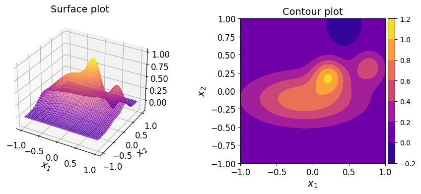
Consider the following two-dimensional function:

\[\begin{split} \begin{align} \mathcal{M}(\boldsymbol{x}) = & 0.75 \exp{\left( -0.25 \left( (x_1 - 2)^2 + (x_2 - 2)^2 \right) \right) } \\ & + 0.75 \exp{\left( -1.00 \left( \frac{(x_1 + 1)^2}{49} + \frac{(x_2 + 1)^2}{10} \right) \right)} \\ & + 0.50 \exp{\left( -0.25 \left( (x_1 - 7)^2 + (x_2 - 3)^2 \right) \right)} \\ & - 0.20 \exp{\left( -1.00 \left( (x_1 - 4)^2 + (x_2 - 7)^2 \right) \right)} \\ \end{align} \end{split}\]

where \(\boldsymbol{x} = (x_1, x_2) \in [-1, 1]^2\).

Note

This function is known in the literature as the Franke function[1]. Here, however, the domain has been redefined to be \([-1, 1]^2\) instead of \([0, 1]^2\).

The function can be defined in Python as follows:

def fun(xx: np.ndarray):
    xx0 = 9 * xx[:, 0]
    xx1 = 9 * xx[:, 1]

    # Compute the (first) Franke function
    term_1 = 0.75 * np.exp(-0.25 * ((xx0 - 2) ** 2 + (xx1 - 2) ** 2))
    term_2 = 0.75 * np.exp(
        -1.00 * ((xx0 + 1) ** 2 / 49.0 + (xx1 + 1) ** 2 / 10.0)
    )
    term_3 = 0.50 * np.exp(-0.25 * ((xx0 - 7) ** 2 + (xx1 - 3) ** 2))
    term_4 = 0.20 * np.exp(-1.00 * ((xx0 - 4) ** 2 + (xx1 - 7) ** 2))

    yy = term_1 + term_2 + term_3 - term_4

    return yy

The surface and contour plots of the function are shown below.

../_images/f3f4d6ffd29a241618a48b82d53aaaa3166f4fe269861a82e516418e59d03181.png

Create an interpolating polynomial#

The steps to create a multidimensional interpolating polynomial in Minterpy from scratch are similar to those used for the one-dimensional case. The steps are:

Define the multi-index set of the polynomial
Construct an interpolation grid
Evaluate the function of interest at the grid points (so-called unisolvent nodes)
Create a polynomial in the Lagrange basis
Transformation from the Lagrange basis to another basis, preferrably the Newton basis, for further manipulation.

As before, we will go through these steps one at a time, highlighting any differences that arise compared to the one-dimensional case.

Define the multi-index set#

As demonstrated in the previous tutorial, multi-index sets in Minterpy are represented by the MultiIndexSet class. You can use the class method from_degree() to create a complete multi-index set for a given spatial dimension (first argument), polynomial degree and polynomial degree (second argument). For multivariate polynomials, you also need to specify the \(l_p\)-degree (\(> 0.0\)) of the multi-index set (third argument).

A complete multi-index set with spatial dimension \(m\), polynomial degree \(n\), and \(l_p\)-degree \(p\) denoted by \(A_{m, n, p}\) includes all multi-indices \(\boldsymbol{\alpha}\) that satisfy the condition \(\lVert \boldsymbol{\alpha} \rVert_p \leq n\), specifically

\[ A_{m, n, p} = \{ \boldsymbol{\alpha} \in \mathbb{N}^m: \lVert \boldsymbol{\alpha} \lVert_ p = ( \alpha_1^p + \ldots + \alpha_m^p )^{1/p} \leq n \}. \]

For instance, the complete multi-index set for \(m = 2\), \(n = 5\), \(p = 2.0\):

m = 2
n = 4
p = 2.0
mi = mp.MultiIndexSet.from_degree(m, n, p)
mi

MultiIndexSet(
  array([[0, 0],
         [1, 0],
         [2, 0],
         [3, 0],
         [4, 0],
         [0, 1],
         [1, 1],
         [2, 1],
         [3, 1],
         [0, 2],
         [1, 2],
         [2, 2],
         [3, 2],
         [0, 3],
         [1, 3],
         [2, 3],
         [0, 4]]),
  lp_degree=2.0
)

The set contains the exponents of a multidimensional polynomial. Each column corresponds to the exponents per spatial dimension, while each row indicates the multi-index elements.

To check how many elements the set contains, you can use the built-in len() function:

len(mi)

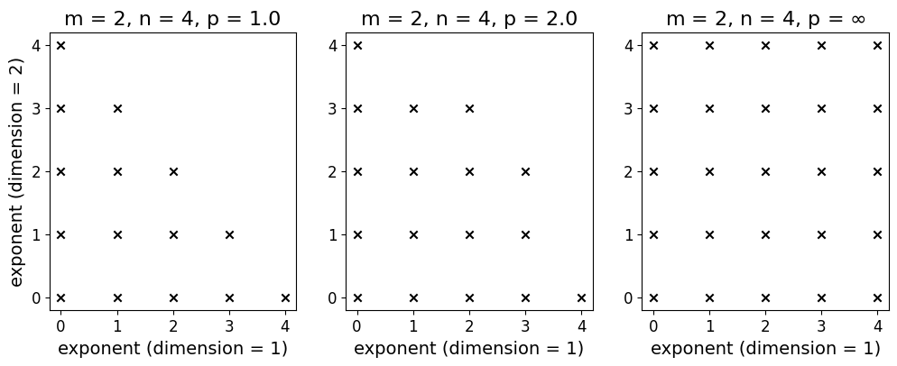
Several common choices for \(l_p\)-degree are \(1.0\) (total-degree set), \(2.0\) (Euclidean-degree set), and \(\infty\) (maximum-degree set). The illustration below shows the difference between these three different choices of \(l_p\)-degree (for the same spatial dimension and polynomial degree) in relation to the exponents as multi-indices.

../_images/b78e76ab316f1715865663c1b9c00d7f8669600bd10499be328693015319f599.png

Construct an interpolation grid#

An interpolating polynomial, one-dimensional or otherwise, lives on an interpolation grid.

To construct an interpolation grid, pass the previously defined multi-index set to the default constructor of the Grid class:

grd = mp.Grid(mi)

The unisolvent nodes associated with the interpolating grid has the same spatial dimension as its defining multi-index set. By default, Minterpy generates unisolvent nodes according to the Leja-ordered Chebyshev-Lobatto points. The unisolvent nodes that correspond to the multi-index set are:

grd.unisolvent_nodes

array([[ 1.00000000e+00, -1.00000000e+00],
       [-1.00000000e+00, -1.00000000e+00],
       [-6.12323400e-17, -1.00000000e+00],
       [ 7.07106781e-01, -1.00000000e+00],
       [-7.07106781e-01, -1.00000000e+00],
       [ 1.00000000e+00,  1.00000000e+00],
       [-1.00000000e+00,  1.00000000e+00],
       [-6.12323400e-17,  1.00000000e+00],
       [ 7.07106781e-01,  1.00000000e+00],
       [ 1.00000000e+00,  6.12323400e-17],
       [-1.00000000e+00,  6.12323400e-17],
       [-6.12323400e-17,  6.12323400e-17],
       [ 7.07106781e-01,  6.12323400e-17],
       [ 1.00000000e+00, -7.07106781e-01],
       [-1.00000000e+00, -7.07106781e-01],
       [-6.12323400e-17, -7.07106781e-01],
       [ 1.00000000e+00,  7.07106781e-01]])

Each row corresponds to two-dimensional grid points; the first and second column contain all the values of the first and second spatial dimension, respectively. These are the points at which the function of interest is evaluated; the results are then used construct an interpolating polynomial.

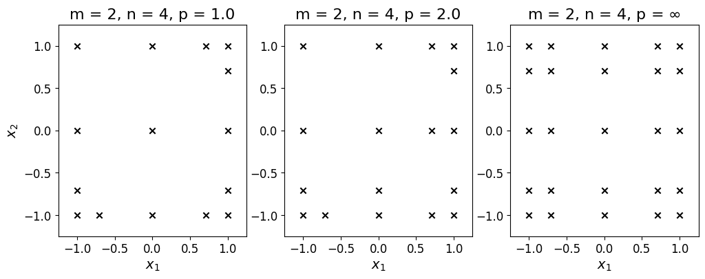
The plots below show three different two-dimensional unisolvent nodes that correspond to three different \(l_p\)-degrees with the same spatial dimension and polynomial degree.

../_images/9ef21995afe07f1d3efdda4709102df49a4228c6294d4377a9aa0c9002d34f2a.png

Evaluate the function at the unisolvent nodes#

An interpolating polynomial satisfies the condition that the polynomial values at the unisolvent nodes coincide with the value of the given function at the same nodes. Calling an instance of Grid with a given function evaluates the function at the unisolvent nodes:

coeffs = grd(fun)
coeffs

array([1.61905391e-04, 3.37547431e-04, 1.22099371e-03, 4.12046496e-04,
       6.92732015e-04, 2.71238400e-05, 9.22305232e-06, 3.46822360e-05,
       5.33538427e-05, 1.07557552e-01, 1.83818849e-01, 7.66420591e-01,
       2.74380251e-01, 5.48517554e-03, 1.14357334e-02, 4.13659227e-02,
       1.12952506e-02])

Note

Make sure that the given function accepts a two-dimensional array whose each column corresponds to the values per spatial dimension.

Create a polynomial in the Lagrange basis#

The function values at the unisolvent nodes are equal to the coefficients of a polynomial in the Lagrange basis \(c_{\mathrm{lag}, \boldsymbol{\alpha}}\):

\[ Q(\boldsymbol{x}) = \sum_{\boldsymbol{\alpha} \in A_{m, n, p}} c_{\mathrm{lag}, \boldsymbol{\alpha}} \Psi_{\mathrm{lag}, \boldsymbol{\alpha}}(\boldsymbol{x}), \]

where \(A_{m, n, p}\) is the complete multi-index set and \(\Psi_{\mathrm{lag}, \boldsymbol{\alpha}}\)’s are the Lagrange basis polynomials, each of which satisfies:

\[ L_{\boldsymbol{\alpha}}(p_{\boldsymbol{\beta}}) = \delta_{\boldsymbol{\alpha}, \boldsymbol{\beta}}, p_{\boldsymbol{\beta}} \in P_{A_{m, n, p}}, \]

where \(\delta{\cdot, \cdot}\) denotes the Kronecker delta.

To create a polynomial in the Lagrange basis from the given grid and coefficients, use the from_grid() class method of LagrangePolynomial class:

lag_poly = mp.LagrangePolynomial.from_grid(grd, coeffs)

Transform to the Newton basis#

Just like the one-dimensional case, to do more with the polynomial in Minterpy, it must first be transformed to the Newton basis such that the polynomial is of the form:

\[ Q(\boldsymbol{x}) = \sum_{\boldsymbol{\alpha} \in A_{m, n, p}} c_{\mathrm{nwt}, \boldsymbol{\alpha}} \, \Psi_{\mathrm{nwt}, \boldsymbol{\alpha}}(\boldsymbol{x}), \]

where \(c_{\mathrm{nwt}, \boldsymbol{\alpha}}\)’s are the coefficients of the polynomial in the multidimensional Newton basis and \(\Psi_{\mathrm{nwt}, \boldsymbol{\alpha}}\)’s are the Newton basis polynomials. The basis polynomial associated with multi-index element \(\boldsymbol{\alpha}\) is defined as follows:

\[ \Psi_{\mathrm{nwt}, \boldsymbol{\alpha}}(\boldsymbol{x}) = \prod_{j = 1}^m \prod_{i = 0}^{\alpha_j - 1} (x_j - p_{i, j}), \]

where \(p_{i, j}\)’s are the interpolation points along dimension \(j\) (i.e., the so-called generating points).

Note

In multiple dimensions (i.e., \(m > 1\)), the generating points / nodes are not the same same as the unisolvent nodes.

As before, to transform a polynomial in the Lagrange basis to a polynomial in the Newton basis, use the LagrangeToNewton class:

nwt_poly = mp.LagrangeToNewton(lag_poly)()

Note

In the above statement, the first part of the call, mp.LagrangeToNewton(lag_poly), creates a transformation instance that converts the given polynomial from the Lagrange basis to the Newton basis.

The second call, which is made without any arguments, performs the transformation and returns the actual NewtonPolynomial instance.

Evaluate the polynomial at a set of query points#

Create a set of random query points in \([-1, 1]^2\):

xx_test = -1 + 2 * np.random.rand(1000, 2)

Then evaluate the original function at these points

yy_test = fun(xx_test)
yy_test[:5]

array([0.41215589, 0.00807249, 0.00082283, 0.16167358, 0.02625827])

Calling an instance of NewtonPolynomial at these query points evaluate the polynomial at the query points:

yy_poly = nwt_poly(xx_test)
yy_poly[:5]

array([ 0.41536034, -0.01848832, -0.01834247,  0.25030834,  0.18142068])

Keep in mind that the input array should have two columns, as the polynomial is two-dimensional.

As expected, evaluating the polynomial at \(1'000\) query points returns an array with \(1'000\) values:

yy_poly.shape

(1000,)

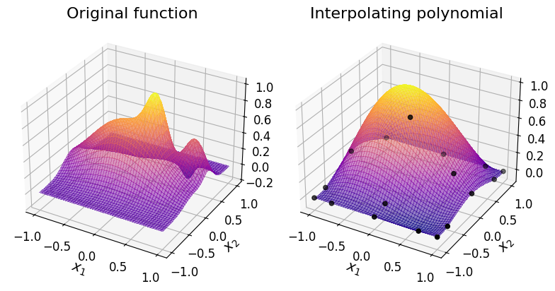
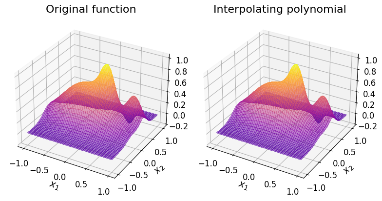
We can compare the surface plot of the original function with that of the interpolating polynomial, which also includes the interpolating nodes:

../_images/64f8b0308268d7bbfcb96fc88a3f97efff06ca98fb8137655111cc54aa2d64ac.png

Assess the accuracy of the polynomial#

As you can see in the plot above, the chosen polynomial degree isn’t sufficient to accurately approximate the original function. The interpolating polynomial misses some of the key features of the original function.

The infinity norm provides a measure of the greatest error of the interpolant over the whole domain. The norm is defined as:

\[ \lVert f - Q \rVert_\infty = \sup_{\boldsymbol{x} \in [-1, 1]^2} \lvert f(\boldsymbol{x}) - Q(\boldsymbol{x}) \rvert \]

The infinity norm of \(Q\) can be approximated using the \(1'000\) test points created above:

np.max(np.abs(yy_test - yy_poly))

np.float64(0.868209330432235)

This number suggests that the interpolating polynomial hasn’t converged yet with the current choices of \(n\) and \(p\).

Assess the empirical convergence of interpolating polynomials#

To assess the convergence of interpolating polynomials, you can once again resort to the high-level function interpolate() as a shortcut to the steps taken above. Let’s investigate the convergence of interpolating polynomials with increasing polynomial degrees and three different choices of \(l_p\)-degrees:

poly_degrees = np.arange(0, 121, 4)
lp_degrees = [1.0, 2.0, np.inf]
yy_poly = np.empty((len(xx_test), len(poly_degrees), len(lp_degrees)))
for i, n in enumerate(poly_degrees):
    for j, p in enumerate(lp_degrees):
        fx_interp = mp.interpolate(fun, spatial_dimension=2, poly_degree=n, lp_degree=p)
        yy_poly[:, i, j] = fx_interp(xx_test)

errors = np.max(np.abs(yy_test[:, np.newaxis, np.newaxis] - yy_poly), axis=0)

The convergence of the error is shown below:

../_images/ea18f4815649806dabcd9ab79bcce93ee7edce49ce4f93e3e8a88563dc51b90e.png

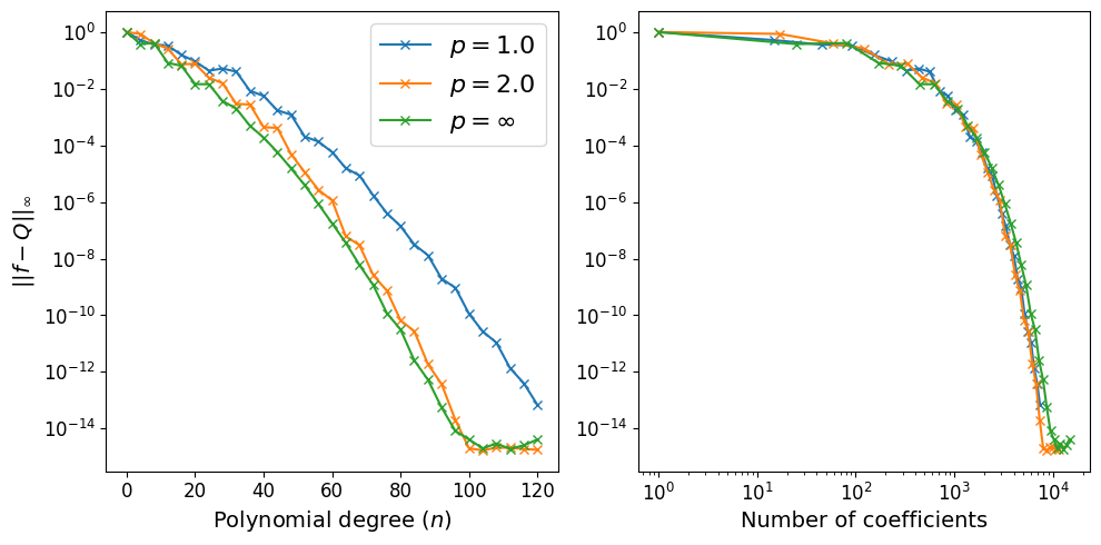
Below are the surface plots of the original function and the interpolating polynomial with \(n = 100\) and \(p = 2.0\), which appears to be numerically converged based on the above plots.

../_images/9db4467e534c72623b28358610083934700ab0705888dcc234850514570ce09f.png

From Interpolant to polynomial#

As explained in the previous tutorial, the callable produced by interpolate() is not a Minterpy polynomial.

There are convenient methods to represent the interpolant in one of the Minterpy polynomials. These methods are summarized in the table below.

Method	Return the interpolant as a polynomial in the…
`to_newton()`	`NewtonPolynomial`
`to_lagrange()`	`LagrangePolynomial`
`to_canonical()`	`CanonicalPolynomial`
`to_chebyshev()`	`ChebyshevPolynomial`

These bases will be the topic of Polynomial Bases and Transformations in-depth tutorial.

To get the interpolating polynomial in the Newton basis, call:

fx_interp.to_newton()

<minterpy.polynomials.newton_polynomial.NewtonPolynomial at 0x7fb861d06410>

Summary#

In this tutorial, you learned how to create a two-dimensional (2D) interpolating polynomial from scratch to approximate a given function then evaluate it at a set of query points in Minterpy.

The steps are:

Define a multi-index set
Construct an interpolation grid
Evaluate the given function on the grid points (i.e., the unisolvent nodes)
Construct an interpolating polynomial in the Lagrange basis
Transform the polynomial into the equivalent Newton basis

As you’ve seen, these steps are similar to the ones in the One-Dimensional Polynomial Interpolation tutorial. Here are some key things to keep in mind when working with multivariate polynomials:

You need to specify the \(l_p\)-degree \(p\) to fully define the multi-index set.
Your function of interest should take a 2D array as input, where each row represents a point in multidimensional space and each column corresponds to a value in each dimension.
When evaluating an interpolating polynomial, make sure your input has the same 2D array structure.

While the example here is two-dimensional, the same principles apply to polynomials in higher dimensions.

Finally, you saw that for the chosen function, an interpolating polynomial approximate it with sufficiently high polynomial degree.

You’ve now learned how to construct and work with interpolating polynomials in Minterpy, whether in one or multiple dimensions.

The next two tutorials will explore additional features and capabilities of Minterpy polynomials.