Polynomial Regression with Minterpy#

The polynomials you’ve worked with in these tutorials are designed to approximate functions of interest by using values at specific, strategically chosen points that form unisolvent nodes. This implies that you have the flexibility to evaluate the function at these selected points within its domain.

However, situations may arise where function values are available only at arbitrary, scattered points across the domain. In such cases, you cannot select the evaluation points freely. Despite this limitation, it is still possible to derive a polynomial that best fits the scattered data using the least squares method.

In this in-depth tutorial, you’ll learn how to perform polynomial regression in Minterpy to construct a polynomial that fits scattered data. This process involves finding the polynomial that minimizes the error between the observed values and the values predicted by the polynomial.

As usual, before you begin, you’ll need to import the necessary packages to follow along with this guide.

import minterpy as mp
import numpy as np
import matplotlib.pyplot as plt

Motivating problem#

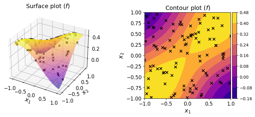
Consider the following two-dimensional transcendental functions:

\[ f(\boldsymbol{x}) = \frac{1}{\sqrt{2}} \left( f_1(x_1) f_1(x_2) + f_2(x_1) f_2(x_2) \right), \]

where

\[\begin{split} \begin{aligned} f_1(x) & = \frac{1}{\pi^{1/4}} e^{-x^2/2} \\ f_2(x) & = \frac{2 x}{\sqrt{\pi}} f_1(x), \end{aligned} \end{split}\]

and \(\boldsymbol{x} = (x_1, x_2) \in [-1, 1]^2\).

Given a dataset of pairs \(\{ (\boldsymbol{x}^{(i)}, y^{(i)}) \}_{i = 1}^N\), your task is to construct a polynomial that approximates the function.

First, define the above functions in Python:

def fun_1(x):
    return 1 / np.pi**(1 / 4) * np.exp(-0.5 * x**2)

def fun_2(x):
    return fun_1(x) * (2 * x) / np.sqrt(np.pi)

def fun(xx):
    return 1 / np.sqrt(2) * fun_1(xx[:, 0]) * fun_1(xx[:, 1]) + fun_2(xx[:, 0]) * fun_2(xx[:, 1])

Then, generate the dataset randomly, say with \(100\) points:

rng = np.random.default_rng(9271)
xx_train = -1 + 2 * rng.random((100, 2))
yy_train = fun(xx_train)

The plots of the function along with the given dataset are shown below.

../_images/56ea17af53dfe6cb88b463d619deb466b7825671349f27a38b0e0dfce80f9aa9.png

Polynomial regression#

In polynomial regression, we construct a linear system of equations as follows:

\[ \boldsymbol{R} \, \boldsymbol{c} = \boldsymbol{y}, \]

where \(\boldsymbol{R}\), \(\boldsymbol{c}\), \(\boldsymbol{y}\) are the regression matrix, the vector of polynomial coefficients, and the vector of output data, respectively.

Each column of the regression matrix \(\boldsymbol{R}\) is obtained by evaluating each of the monomials of the chosen polynomial basis at the each input data.

The goal of polynomial regression is to estimate \(\boldsymbol{c}\) given \(\{ (\boldsymbol{x}^{(i)}, y^{(i)}) \}_{i = 1}^N\) such that chosen polynomial becomes fully determined.

Define a polynomial model#

Following the steps shown in the previous examples, defining a polynomial starts with defining the underlying multi-index set.

For instance, you may define a multi-index set of polynomial degree \(8\) and \(l_p\)-degree \(2.0\):

mi = mp.MultiIndexSet.from_degree(2, 8, 2.0)

Make sure that the size of the multi-index set is at least smaller than the available data points.

len(mi)

Create an ordinary regression polynomial#

The OrdinaryRegression class is used as an interface between polynomials that you’ve seen before and regression polynomial.

To create an instance of OrdinaryRegression, pass the multi-index set to the default constructor:

reg_poly = mp.OrdinaryRegression(mi)

By default, if not specified, an underlying interpolating grid is created using Leja-ordered Chebyshev-Lobatto points. Additionally, the underlying polynomial is, by default, represented in the Lagrange basis. In other words, ordinary least squares will subsequently be used to estimate the coefficients of the polynomial in the Lagrange basis.

Fit the regression polynomial#

You have so far constructed a regression polynomial by defining the structure of the underlying polynomial. For now, however, its coefficients remain unknown.

reg_poly.coeffs is None

True

The polynomial coefficients are obtained by solving the following least-squares problem (ordinary least-squares):

\[ \hat{\boldsymbol{c}} = \underset{\boldsymbol{c}}{\mathrm{arg min}} \lVert \boldsymbol{R} \boldsymbol{c} - \boldsymbol{y} \rVert_2^2 \]

where: \(\lVert \cdot \rVert_2^2\) denotes the square of the Euclidean norm.

You can use the method fit() to solve the above problem on the given regression polynomial instance. The method requires a pair of inputs and the corresponding output are required. As these are already constructed above:

reg_poly.fit(xx_train, yy_train)

/home/runner/work/minterpy/minterpy/src/minterpy/schemes/barycentric/operators.py:50: UserWarning: building a full transformation matrix from a barycentric transformation. this is inefficient.
  warn(

Note that the call to fit() alters the instance in-place; once the call is concluded, the coefficients are available:

reg_poly.coeffs[:10]  # the first 10

array([-0.11473161,  0.41097058,  0.24196861, -0.05085656,  0.42838383,
        0.37984464,  0.06996035, -0.10282655,  0.42058672,  0.41146145])

Evaluate the regression polynomial#

Once fitted, you can evaluate the instance at a set of query points.

For instance:

reg_poly(
    np.array([
        [-1., 1.],
        [-0.5, 0.0],
        [0.0, 0.5],
    ])
)

array([-0.11748932,  0.3520634 ,  0.35206581])

Verify the fitted polynomial#

You can also check several measures that indicate the quality of the fitted polynomial by calling the show():

reg_poly.show()

Ordinary Polynomial Regression
------------------------------
Spatial dimension: 2
Poly. degree     : 8
Lp-degree        : 2.0
Origin poly.     : <class 'minterpy.polynomials.lagrange_polynomial.LagrangePolynomial'>
Error                     Absolute     Relative
L-inf Regression Fit   2.57395e-06  1.77514e-05
L2 Regression Fit      8.05418e-13  3.83077e-11
LOO CV                 2.59071e-10  1.23220e-08

The three measures of fitting error are:

Infinity norm (L-inf)
Euclidean norm (L2)
Leave-one-out cross validation error (LOO CV)

Note that for L2 and LOO CV the errors are still squared.

For L2 and LOO CV the relative errors are the absolute errors normalized by the variance of the output in the dataset. For L-inf the relative error is the absolute error normalized by the standard deviation of the output in the dataset.

These fitting error measures are solely based on the training dataset. You should view them critically; small values do not necessarily means highly accurate regression polynomial as they tend to underestimate the generalization error (i.e., error based on the unseen data). That being said, the LOO-CV error is usually a more robust estimate of the generalization error than the other two.

To estimate the generalization error in L2 sense:

xx_test = -1 + 2 * rng.random((10000, 2))
yy_test = fun(xx_test)
print(np.mean((yy_test - reg_poly(xx_test))**2))

1.2993877590648122e-08

The plots below show the surface, contour, and the error plot for the regression polynomial.

Show code cell source Hide code cell source

from mpl_toolkits.axes_grid1 import make_axes_locatable

# --- Create 2D data
xx_1d = np.linspace(-1.0, 1.0, 500)[:, np.newaxis]
mesh_2d = np.meshgrid(xx_1d, xx_1d)
xx_2d = np.array(mesh_2d).T.reshape(-1, 2)
yy_fun_2d = fun(xx_2d)
yy_reg_2d = reg_poly(xx_2d)
yy_err_2d = np.abs(yy_fun_2d - yy_reg_2d)

# --- Create two-dimensional plots
fig = plt.figure(figsize=(15, 5))

# Surface
axs_1 = plt.subplot(131, projection='3d')
axs_1.plot_surface(
    mesh_2d[0],
    mesh_2d[1],
    yy_reg_2d.reshape(500, 500).T,
    linewidth=0,
    cmap="plasma",
    antialiased=False,
    alpha=0.4,
)
axs_1.scatter(
    xx_train[:, 0],
    xx_train[:, 1],
    yy_train,
    color="k",
    marker="x",
)
axs_1.set_xlabel("$x_1$", fontsize=14)
axs_1.set_ylabel("$x_2$", fontsize=14)
axs_1.set_title("Surface plot ($Q$)", fontsize=14)
axs_1.tick_params(axis='both', which='major', labelsize=12)

# Contour
axs_2 = plt.subplot(132)
cf = axs_2.contourf(
    mesh_2d[0], mesh_2d[1], yy_reg_2d.reshape(500, 500).T, cmap="plasma"
)
axs_2.scatter(xx_train[:, 0], xx_train[:, 1], color="k", marker="x")
axs_2.set_xlabel("$x_1$", fontsize=14)
axs_2.set_ylabel("$x_2$", fontsize=14)
axs_2.set_title("Contour plot ($Q$)", fontsize=14)
divider = make_axes_locatable(axs_2)
cax = divider.append_axes('right', size='5%', pad=0.05)
fig.colorbar(cf, cax=cax, orientation='vertical')
axs_2.axis('scaled')
axs_2.tick_params(axis='both', which='major', labelsize=12)

# Contour Eror
axs_3 = plt.subplot(133)
cf = axs_3.contourf(
    mesh_2d[0], mesh_2d[1], yy_err_2d.reshape(500, 500).T, cmap="plasma"
)
axs_3.scatter(xx_train[:, 0], xx_train[:, 1], color="k", marker="x")
axs_3.set_xlabel("$x_1$", fontsize=14)
axs_3.set_ylabel("$x_2$", fontsize=14)
axs_3.set_title("Error ($| f - Q |$)", fontsize=14)
divider = make_axes_locatable(axs_3)
cax = divider.append_axes('right', size='5%', pad=0.05)
fig.colorbar(cf, cax=cax, orientation='vertical')
axs_3.axis('scaled')
axs_3.tick_params(axis='both', which='major', labelsize=12)

fig.tight_layout()

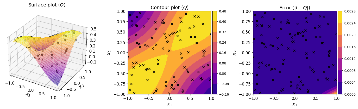
../_images/2016379e8fc23d4a7038a140069f5eb625aa6f24b0b84d3126358ade1d04c658.png

The plots show that the regression polynomial captures the overall behavior of the original function well. This indicates that the chosen polynomial structure and the available data are sufficient. Furthermore, the error plot shows that the differences between the regression polynomial and the original function are small across the function domain.

Closing remark#

Once fitted, a regression polynomial is fully determined. In particular, the eval_poly property of the instance is a Minterpy polynomial you’ve already familiar. You can carry out arithmetic as well as calculus operations on it.

reg_poly.eval_poly

<minterpy.polynomials.newton_polynomial.NewtonPolynomial at 0x7f8c1c085f60>

By default, the evaluation polynomial is set to be a polynomial in the Newton basis.

Summary#

In this tutorial, you’ve learned how to perform polynomial regression using Minterpy. This is particularly useful when working with a dataset consisting of input–output pairs, especially when the underlying function is unknown or inaccessible.

Polynomial regression in Minterpy is facilitated through the OrdinaryRegression class. The steps to construct a regression polynomial are as follows:

Determine the structure of the underlying polynomial by specifying the multi-index set.
Create an instance of OrdinaryRegression based on the defined polynomial structure.
Fit the instance with the given dataset using the fit() method.
Verify the regression polynomial using the show() method.

Once fitted, the resulting instance is callable, allowing you to evaluate it at any set of query points by passing these points directly to the instance.

Finally, you can also access the underlying fitted polynomial from the eval_poly property of the instance. This polynomial is a Minterpy polynomial, so you can apply a variety of arithmetic and calculus operations on it, as covered in the previous tutorials.

Congratulations on completing this series of Minterpy in-depth tutorials!

You should now be familiar with the main features of Minterpy. We hope you find Minterpy valuable for your work!