
Multiply Grid Instances#
import matplotlib.pyplot as plt
import minterpy as mp
import numpy as np
This guide demonstrates how to multiply instances of Grid and the expected outcome of such an operation. The multiplication between two instances of Grid may be carried out via the operator *.
The result of a multiplication between two instances of Grid is another instance of Grid whose underlying multi-index set is the product of the index sets of the operands. This Grid instance
can support interpolation polynomials that are the product of polynomials that live on either Grid operands.
To know more about the multi-index set multiplication in Minterpy, see the relevant example.
When multiplying two instances of Grid note the following caveats:
If a generating function is defined in both instances, then the instances can be multiplied only if the generating functions are compatible, i.e., they are the same function. defined in both instances.
Without a generating function, two instances can be multiplied only if the generating points are compatible, i.e., they have the same values up to a common dimension (or columns).
Example: Instances with the same dimension#
As a motivating example, consider multiplying two two-dimensional interpolation grids:
The first grid has a complete multi-index set with respect to a polynomial degree \(2\) and \(l_p\)-degree \(2.0\)
the second grid has a complete multi-index set with respect to a polynomial degree \(3\) and \(l_p\)-degree \(1.0\).
Both interpolation grids have points according to the Leja-ordered Chebyshev-Lobatto points (the default in Minterpy).
First, create the instances of Grid according to the above specification:
grd_1 = mp.Grid.from_degree(2, 2, 2.0)
grd_2 = mp.Grid.from_degree(2, 3, 1.0)
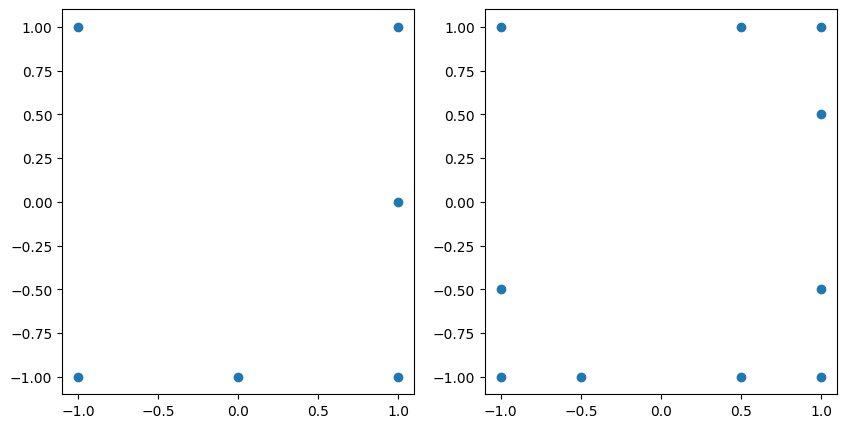
The unisolvent nodes that correspond to these are shown below:
fig, axs = plt.subplots(1, 2, figsize=(10, 5))
axs[0].scatter(grd_1.unisolvent_nodes[:, 0], grd_1.unisolvent_nodes[:, 1])
axs[1].scatter(grd_2.unisolvent_nodes[:, 0], grd_2.unisolvent_nodes[:, 1]);
The product Grid can be obtained as follows:
grd_prod = grd_1 * grd_2
And the resulting unisolvent nodes are shown below:
plt.scatter(grd_prod.unisolvent_nodes[:, 0], grd_prod.unisolvent_nodes[:, 1]);
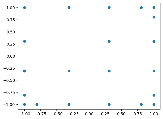
Notice that the underlying multi-index set follows the convention adopted
for the multiplication of MultiIndexSet:
print(grd_prod.multi_index)
MultiIndexSet(m=2, n=5, p=2.0)
[[0 0]
 [1 0]
 [2 0]
 [3 0]
 [4 0]
 [5 0]
 [0 1]
 [1 1]
 [2 1]
 [3 1]
 [4 1]
 [0 2]
 [1 2]
 [2 2]
 [3 2]
 [0 3]
 [1 3]
 [2 3]
 [0 4]
 [1 4]
 [0 5]]
Example: Instances with different dimension#
Grids of different spatial dimensions may also be multiplied with each other. For instance, consider multiplying the following interpolation grids:
the first grid is a one-dimensional grid whose a complete multi-index set with respect to a polynomial degree \(4\)
the second grid is a two-dimensional grid whose a complete multi-index set with respect to a polynomial degree \(2\) and \(l_p\)-degree \(1.0\).
Both interpolation grids have points according to the Leja-ordered Chebyshev-Lobatto points (the default in Minterpy).
The product grid will have the same spatial dimension as that of the operands with the largest dimension.
First, create the two instances of Grid following the above specification:
grd_1 = mp.Grid.from_degree(1, 4, 1.0)
grd_2 = mp.Grid.from_degree(2, 2, 1.0)
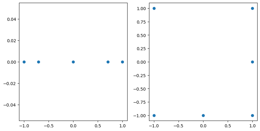
The unisolvent nodes that correspond to these are shown below:
fig, axs = plt.subplots(1, 2, figsize=(10, 5))
axs[0].scatter(grd_1.unisolvent_nodes[:, 0], np.zeros(len(grd_1.multi_index)))
axs[1].scatter(grd_2.unisolvent_nodes[:, 0], grd_2.unisolvent_nodes[:, 1]);
The product Grid can be obtained as follows:
grd_prod = grd_1 * grd_2
And the resulting unisolvent nodes are shown below:
plt.scatter(grd_prod.unisolvent_nodes[:, 0], grd_prod.unisolvent_nodes[:, 1]);
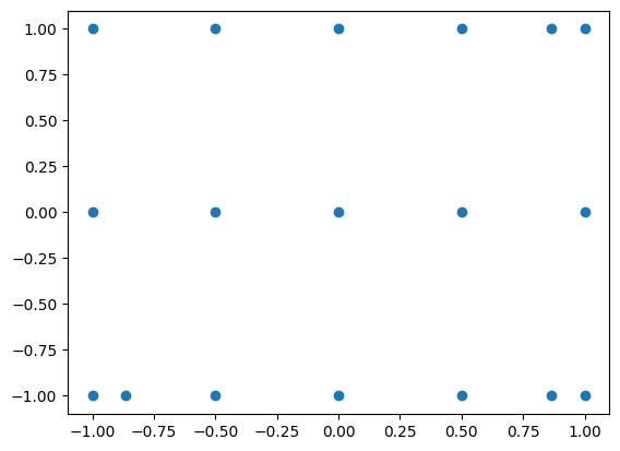
As expected the resulting Grid is two-dimensional according to the largest dimension of the operands. The resulting multi-index set is shown below:
print(grd_prod.multi_index)
MultiIndexSet(m=2, n=6, p=1.0)
[[0 0]
 [1 0]
 [2 0]
 [3 0]
 [4 0]
 [5 0]
 [6 0]
 [0 1]
 [1 1]
 [2 1]
 [3 1]
 [4 1]
 [5 1]
 [0 2]
 [1 2]
 [2 2]
 [3 2]
 [4 2]]