Integrate a One-Dimensional Polynomial

import numpy as np
import minterpy as mp
import matplotlib.pyplot as plt

import warnings
warnings.filterwarnings('ignore')

A definite integration operation may be carried for fully-specified Minterpy polynomials. This guide explains how to carry out a definite integration on a one-dimensional polynomial interpolant in different bases.

Motivating example

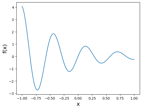
Consider the following one-dimensional damped sine function:

\[ f(x) = e^{-1.4 x} \sin{(3.5 \pi x)},\;\; x \in [-1, 1]. \]

An estimated value of this integral is \(0.0490183\).

Define the function in Python as follows:

def fun(xx):
    return np.exp(-1.4 * xx) * np.sin(3.5 * np.pi * xx)

The plot of the function is shown in the figure below:

xx = np.linspace(-1, 1, 10000)
yy = fun(xx)

plt.plot(xx, yy)
plt.xlabel("x", fontsize=16)
plt.ylabel("f(x)", fontsize=16);

Polynomial interpolation

In this guide, we are going to create a polynomial interpolant in Minterpy from scratch in four steps:

1. Define the multi-index set

2. Create the interpolation grid (of unisolvent nodes)

3. Evaluate the function on the grid

4. Create a polynomial interpolant in Lagrange basis

A polynomial interpolant of a given degree may be created using the Lagrange basis. First, create the multi-index set:

mi = mp.MultiIndexSet.from_degree(spatial_dimension=1, poly_degree=30, lp_degree=1.0)

We select a high enough polynomial degree to sufficiently interpolate the function. Then, create the interpolation grid given multi-index set:

grd = mp.Grid(multi_index=mi)

The grid contains unisolvent nodes on which the function should be evaluated as the coefficients of a polynomial in the Lagrange basis:

lag_coeffs = fun(grd.unisolvent_nodes)

Finally, a polynomial interpolant in Lagrange basis is created from the multi-index set and the set of coefficients:

lag_poly = mp.LagrangePolynomial(multi_index=mi, coeffs=lag_coeffs)

Note

In Minterpy, polynomials in the Lagrange basis cannot be directly evaluated. To evaluate an interpolating polynomial, the Newton basis is recommended.

Integration over the domain \([-1, 1]\)

The method integrate_over() integrates the polynomial over the default domain of \([-1, 1]\):

int_value = lag_poly.integrate_over()
int_value

0.049018277818983005

Integration over specified bounds

The bounds of the integration may be specified. For instance, to integrate the polynomial over \([-1, 0]\), provide the lower and upper bounds of the integration as follows:

lag_poly.integrate_over([-1, 0])

-0.04328650053261674

Similarly, to integrate the polynomial over \([0, 1]\):

lag_poly.integrate_over([0, 1])

0.09230477835159537

Integration in different bases

The integration may also be carried out on the polynomial in different bases. The same method integrate_over() is used. Below is the integration in the Newton basis:

nwt_poly = mp.LagrangeToNewton(lag_poly)()
nwt_poly.integrate_over()

0.0490182778189841

And in the canonical basis:

can_poly = mp.LagrangeToCanonical(lag_poly)()
can_poly.integrate_over()

0.049018433527192186

Warning

The integration of polynomials in the canonical basis having a high polynomial degree is not recommended as it may suffer from a severe instability.