
Create a Grid from an Array of Generating Points#
import numpy as np
import minterpy as mp
import matplotlib.pyplot as plt
Minterpy interpolating polynomials (i.e., in the Lagrange or Newton basis) lives on a grid that holds the so-called unisolvent nodes. An interpolating multi-dimensional polynomial of a given multi-index set of exponents is uniquely determined on the corresponding unisolvent nodes.
An instance of Grid can be constructed via different constructors:
Grid.from_points(): create an instance with an array of generating points (this page)Grid.from_function(): create an instance with a generating function (see the example)Grid.from_degree(): create an instance with a complete multi-index set (see the example)Grid.from_value_set(): create an instance based on an array of generating values (see the example)
This guide provides an example on how to construct a Grid instance based
on a given array of generating points using the from_points() method.
About generating points#
Valid generating points to construct an instance of Grid are given as
a two-dimensional array of floats that must additionally satisfy
the following conditions:
the values must be in \([-1, 1]^m\), regardless of the domain assigned to the grid.
the shape must be \((n + 1, m)\) where \(n\) is the maximum polynomial degree across all dimensions and \(m\) is the spatial dimension. Each column of the array is the one-dimensional interpolation points associated with that dimension.
each column of the array must have unique values (no repeats).
the number of rows of the array must be equal to or larger than the maximum exponents of the grid’s multi-index set in any dimension.
About from_points() factory method#
The method from_points() of the Grid class returns an instance of Grid
based on a given array of generating points.
The method accepts two mandatory arguments, namely, the multi-index set of exponents that defines the polynomials that grid can support, and the generating points as required by the multi-index set.
As explained above, the array of generating points must satisfy several conditions for it to be valid.
The method also accepts an optional domain argument. If not specified the domain defaults to the internal reference domain \([-1, 1]^m\). As noted above, regardless of the specified domain, the generating points must always be in \([-1, 1]^m\).
The from_points() method is a shortcut to create a grid with a given multi-index set
and a specific array of generating points.
Example: Two-dimensional interpolation grid#
Create an interpolation grid in \([-1, 1]^2\) to support two-dimensional polynomials having a multi-index set \(A = \{ (0, 0), (1, 0), (2, 0), (0, 1), (1, 1), (0, 2), (1, 2), (0, 3), (1, 3) \}\) (defined with respect to \(l_p\)-degree \(1.0\)). The interpolation grid has Leja-ordered Chebyshev-Lobatto points in the first dimension and the Leja points in the second dimension.
Multi-index set#
Create an instance of MultiIndexSet following the above specification:
exponents = np.array([
    [0, 0],
    [1, 0],
    [2, 0],
    [0, 1],
    [1, 1],
    [0, 2],
    [1, 2],
    [0, 3],
    [1, 3],
])
mi = mp.MultiIndexSet(exponents, lp_degree=1.0)
print(mi)
MultiIndexSet(m=2, n=4, p=1.0)
[[0 0]
 [1 0]
 [2 0]
 [0 1]
 [1 1]
 [0 2]
 [1 2]
 [0 3]
 [1 3]]
Generating points#
The generating points as required by the grid are given as follows:
gen_points = np.array([
    [-1., 0. ],
    [ 1., -1. ],
    [-0.5, 1.0],
    [ 0.5, 0.57735035],
])
Because the maximum exponents in the multi-indices across all dimensions is \(3\), the required number of points is \(3 + 1 = 4\) per column.
As shown above, the distribution of points per column does not have to be identical. In this particular case, each column is based on different one-dimensional interpolation points. The generating points, however, must have unique values per column.
Grid instance#
An instance of Grid given the multi-index set and the array of generating points
can be constructed via from_points() method as follows:
grd = mp.Grid.from_points(mi, gen_points)
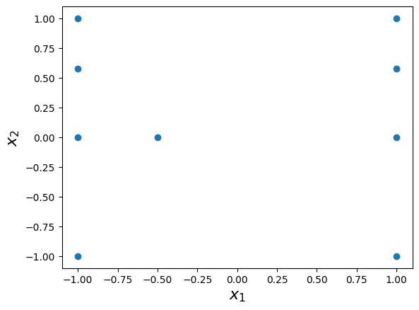
The grid has the following unisolvent nodes:
print(grd.unisolvent_nodes)
[[-1.          0.        ]
 [ 1.          0.        ]
 [-0.5         0.        ]
 [-1.         -1.        ]
 [ 1.         -1.        ]
 [-1.          1.        ]
 [ 1.          1.        ]
 [-1.          0.57735035]
 [ 1.          0.57735035]]
The two-dimensional interpolation grid is plotted below:
plt.scatter(grd.unisolvent_nodes[:, 0], grd.unisolvent_nodes[:, 1])
plt.xlabel("$x_1$", fontsize=16)
plt.ylabel("$x_2$", fontsize=16);
Note
Regardless of the specified domain, the unisolvent nodes are stored in the internal reference domain \([-1, 1]^m\). When the domain is not \([-1, 1]^m\), Minterpy automatically transforms the nodes to the specified domain before passing them to the function, for example, when calling
grid(func).