
Create a Grid with a Complete Multi-Index Set#
import numpy as np
import minterpy as mp
import matplotlib.pyplot as plt
Minterpy interpolating polynomials (i.e., in the Lagrange or Newton basis) lives on a grid that holds the so-called unisolvent nodes. An interpolating multi-dimensional polynomial of a given multi-index set of exponents is uniquely determined on the corresponding unisolvent nodes.
An instance of Grid can be constructed via different constructors:
Grid.from_degree(): create an instance with a complete multi-index set (this page)Grid.from_function(): create an instance with a generating function (see the example)Grid.from_points(): create an instance with an array of generating points (see the example)Grid.from_value_set(): create an instance based on an array of generating values (see the example)
This guide provides an example on how to construct a Grid instance with
a complete multi-index set using the from_degree() method.
About complete multi-index sets#
A complete multi-index set with respect to spatial dimension \(m\), polynomial degree \(n\), and \(l_p\)-degree \(p\) denoted by \(A_{m, n, p}\) contains all the exponents \(\boldsymbol{\alpha} = (\alpha_1, \ldots, \alpha_m) \in \mathbb{N}^m\) such that the \(l_p\)-norm \(\lVert \boldsymbol{\alpha} \rVert_p \leq n\) holds.
A complete multi-index set is a typical way (but by no means, the only way) to define a multi-index set of exponents in Minterpy.
About from_degree() factory method#
The method from_degree() of the Grid class returns an instance of Grid
based on the specification of a complete multi-index set and optionally,
the generating function and the generating points.
The method accepts the following arguments:
spatial_dimension(\(m\)): the dimension of the multi-index set and subsequently, the grid.poly_degree(\(n\)): the polynomial degree of the set.lp_degree(\(p\)): the \(l_p\)-degree with respect to which the complete multi-index set is defined.generating_function: the generating function to create an array of generating points required by the complete multi-index set. This argument is optional; if not specified, the default Leja-ordered Chebyshev-Lobatto generating function is selected. For detail regarding a valid generating function, see the corresponding example.generating_points: the generating points of the interpolation grid. This argument is optional; if not specified, the points are generated by the generating function as required. For detail regarding valid generating points, see the corresponding example.domain: the user-defined domain of the interpolation grid. This argument is optional; if not specified, the domain defaults to the internal reference domain \([-1, 1]^m\). Regardless of the specified domain, however, generating points must lie in \([-1, 1]^m\) and any generating function must return values in \([-1, 1]^m\).
The from_degree() method is a shortcut for constructing a grid that corresponds
to a complete multi-index set; it avoids the separate construction of a complete
MultiIndexSet instance that is then passed to the other constructors of the
Grid class.
Example: Two-dimensional interpolation grid#
Create an interpolation grid that can support two-dimensional polynomials defined by a complete multi-index set of polynomial degree \(3\) with respect to \(l_p\)-degree \(\infty\) and with Leja-ordered Chebyshev-Lobatto points as the generating points.
An instance of Grid that satisfies the above condition can be created using
from_degree() method as follows:
grd = mp.Grid.from_degree(
    spatial_dimension=2,
    poly_degree=3,
    lp_degree=np.inf,
)
As the Leja-ordered Chebyshev-Lobatto points are the generating function selected by default, no specification is required.
The grid has the following unisolvent nodes:
print(grd.unisolvent_nodes)
[[ 1.  -1. ]
 [-1.  -1. ]
 [ 0.5 -1. ]
 [-0.5 -1. ]
 [ 1.   1. ]
 [-1.   1. ]
 [ 0.5  1. ]
 [-0.5  1. ]
 [ 1.  -0.5]
 [-1.  -0.5]
 [ 0.5 -0.5]
 [-0.5 -0.5]
 [ 1.   0.5]
 [-1.   0.5]
 [ 0.5  0.5]
 [-0.5  0.5]]
The two-dimensional interpolation grid is plotted below:
plt.scatter(grd.unisolvent_nodes[:, 0], grd.unisolvent_nodes[:, 1])
plt.xlabel("$x_1$", fontsize=16)
plt.ylabel("$x_2$", fontsize=16);
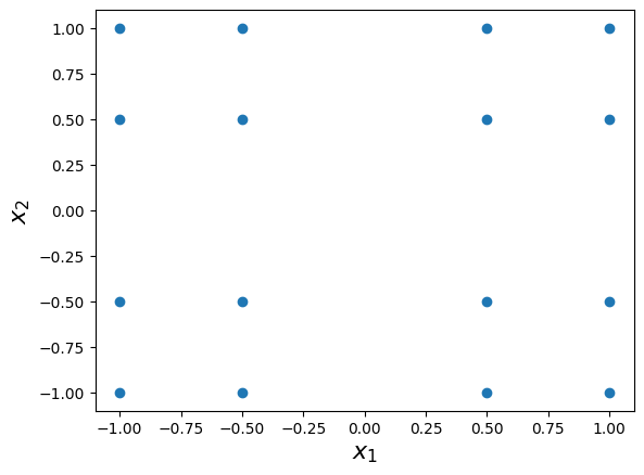
This interpolation grid corresponds to the full tensorial grid of two-dimensional polynomials with polynomial degree of \(3\).
Note
Regardless of the specified domain, the unisolvent nodes are stored in the internal reference domain \([-1, 1]^m\). When the domain is not \([-1, 1]^m\), Minterpy automatically transforms the nodes to the specified domain before passing them to the function, for example, when calling
grid(func).