Add Exponents to a Grid

import minterpy as mp
import numpy as np
import matplotlib.pyplot as plt

An additional multi-index exponent or a set of multi-indices may be added to a Grid instance. A new instance of Grid is returned with the expanded underlying multi-index set. The Grid may then support a larger space of interpolant polynomials.

The logic behind adding elements to a grid in Minterpy follows the logic of adding the elements to a multi-index set. See Add Exponents to a Multi-Index Set for more details.

Motivating example

Consider a two-dimensional Leja-ordered Chebyshev-Lobatto interpolation grid whose underlying multi-index set is a complete set of spatial dimension \(2\), polynomial degree \(2\), and \(l_p\)-degree \(1.0\):

grd = mp.Grid.from_degree(2, 2, 1.0)

Add an exponent to a Grid instance

The method add_exponents() inserts an exponent to the underlying multi-index set of a Grid instsance. For a single multi-index element, the element may be specified as a one-dimensional array with the spatial dimension as the length.

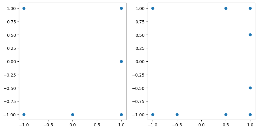
For instance, to add a new exponent \((3, 0)\):

grd_added_1 = grd.add_exponents(np.array([3, 0]))

Compare the unisolvent nodes before and after adding the exponent:

fig, axs = plt.subplots(1, 2, figsize=(10, 5))
axs[0].scatter(grd.unisolvent_nodes[:, 0], grd.unisolvent_nodes[:, 1])
axs[1].scatter(
    grd_added_1.unisolvent_nodes[:, 0],
    grd_added_1.unisolvent_nodes[:, 1],
);

Notice that now the grid may support polynomial up to dimension \(3\) in the first dimension.

grd.multi_index

MultiIndexSet(
  array([[0, 0],
         [1, 0],
         [2, 0],
         [0, 1],
         [1, 1],
         [0, 2]]),
  lp_degree=1.0
)

Add a set of exponents to a Grid instance

The method add_exponents() also supports adding multiple multi-index exponents to a Grid instance. The added components must be specified as a two-dimensional integer array with the spatial dimension as the number of columns.

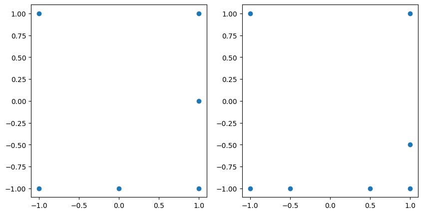
For instance, to add the exponents \(\{ (3, 0), (2, 1), (0, 3) \}\):

grd_added_2 = grd.add_exponents(
    np.array([[3, 0], [2, 1], [0, 3]])
)

Compare the unisolvent nodes before and after adding the new multi-index elements:

fig, axs = plt.subplots(1, 2, figsize=(10, 5))
axs[0].scatter(grd.unisolvent_nodes[:, 0], grd.unisolvent_nodes[:, 1])
axs[1].scatter(
    grd_added_2.unisolvent_nodes[:, 0],
    grd_added_2.unisolvent_nodes[:, 1],
);