
One-Dimensional Polynomial Interpolation#
Welcome to the first in-depth tutorial of Minterpy!
Minterpy is an open source Python package for carrying out numerical tasks with multivariate (multi-dimensional) polynomials. You can do a wide range of arithmetic and calculus operations with Minterpy polynomials.
But how to create such polynomials in the first place?
This tutorial demonstrates how you can create such a polynomial from scratch in the most typical use case: interpolating a function.
Import Minterpy#
After installing Minterpy, you can import it as follows:
import minterpy as mp
The shorthand mp is the convention we, the developer team, like to use; it’s short and recognizable (just like np for NumPy and pd for pandas).
You will also need to import NumPy and Matplotlib to follow along with this guide.
import numpy as np
import matplotlib.pyplot as plt
Motivating function#
Polynomials in Minterpy are typically created by interpolating a function of interest; function approximation by polynomial interpolation is one of the package’s main use cases.
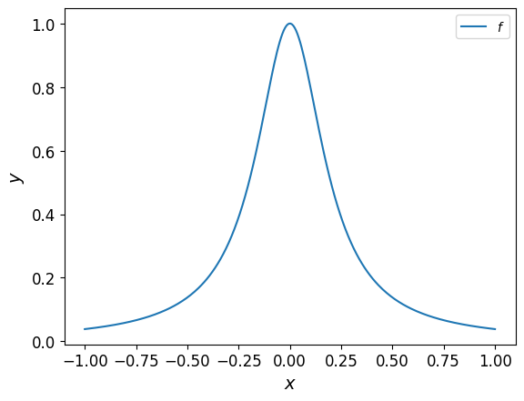
Consider the following one-dimensional function, known as the Runge function:
Define this function in Python:
fun = lambda x: 1 / (1 + 25 * x**2)
The plot of the function is shown below.
Now that you’ve defined your function, you’re ready to create a polynomial that approximates it.
Create an interpolating polynomial#
To create an interpolating polynomial in Minterpy, follow these four main steps:
Define the multi-index set: Specify the multi-index set that determines the structure of the polynomial.
Construct an interpolation grid: Create an interpolation grid, which consists of the points at which the function of interest will be evaluated.
Evaluate the function at the grid points: Compute the function values at the grid points, also known as the unisolvent nodes
Create a polynomial in the Lagrange basis: Construct the interpolating polynomial in the Lagrange basis based on the evaluated points.
To perform additional operations with the interpolating polynomial, such as evaluating it at a set of query points, follow this extra step:
Transform the polynomial to another basis: Change the basis of the interpolating polynomial from the Lagrange basis to another basis, typically the Newton basis, which is well-suited for evaluation and manipulation.
Let’s go through these steps one at a time.
Define a multi-index set#
In Minterpy, the exponents of a multivariate polynomial are represented using multi-indices within a set known as the multi-index set. This set generalizes the notion of polynomial degree to multiple dimensions. For more details, see the relevant section of the documentation.
Even though our function is one-dimensional, defining the multi-index set (in this case, of dimension \(1\)) is still the first step of constructing a Minterpy polynomial.
In Minterpy, multi-index sets are represented by the MultiIndexSet class.
You can create a complete multi-index set using the class method from_degree(), which requires the spatial dimension (first argument) and the polynomial degree (second argument). The third argument, the \(l_p\)-degree, does not affect the result for one-dimensional polynomials.
To construct a one-dimensional multi-index set of polynomial degree \(10\), type:
mi = mp.MultiIndexSet.from_degree(1, 10)
This produces the following instance:
mi
MultiIndexSet(
  array([[ 0],
         [ 1],
         [ 2],
         [ 3],
         [ 4],
         [ 5],
         [ 6],
         [ 7],
         [ 8],
         [ 9],
         [10]]),
  lp_degree=2.0
)
Construct an interpolation grid#
An interpolation grid defines the set of points on which an interpolating polynomial is built. The bases of interpolating polynomials, such as the Lagrange or Newton bases, are built with respect to these grids.
In Minterpy, interpolation grids are represented by the Grid class.
The default constructor allows you to create an interpolation grid for a specified multi-index set (the first argument).
To create an interpolation grid for the previously defined multi-index set, use the following command:
grd = mp.Grid(mi)
In simple terms, the multi-index set of an interpolation grid determines the structure of multivariate polynomials that the grid can support.
A key property of a Grid instance is unisolvent_nodes (i.e., interpolating nodes or grid points).
These nodes are crucial because they uniquely determine the interpolating polynomial given the multi-index set.
By default, Minterpy generates unisolvent nodes based on the Leja-ordered Chebyshev-Lobatto points.
For the chosen polynomial degree, these nodes are:
grd.unisolvent_nodes
array([[ 1.00000000e+00],
       [-1.00000000e+00],
       [-6.12323400e-17],
       [ 5.87785252e-01],
       [-5.87785252e-01],
       [ 8.09016994e-01],
       [-8.09016994e-01],
       [ 3.09016994e-01],
       [-3.09016994e-01],
       [ 9.51056516e-01],
       [-9.51056516e-01]])
which are distributed as follows:
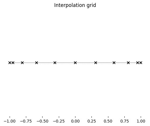
Notice that there are more points near the boundaries of the domain.
Note
No domain is specified when constructing the grid above. In that case, Minterpy defaults to the internal reference domain \([-1, 1]^m\). o learn how to define a custom domain, see Multivariate Polynomial Interpolation.
Unisolvent nodes are always expressed in the canonical domain \([-1, 1]^m\), regardless of the user-defined domain.
Evaluate the function at the unisolvent nodes#
An interpolating polynomial \(Q\) of a function \(f\) on \([-1, 1]\) is a polynomial that satisfies the following condition:
where \(P_A = \{ p_{\alpha}: \alpha \in A \}\) is the set of unisolvent nodes.
The function values at the unisolvent nodes are therefore crucial for constructing an interpolating polynomial.
In Minterpy, calling an instance of Grid with a given function evaluates the function at the unisolvent nodes and returns the values as an array
coeffs = grd(fun)
coeffs
array([[0.03846154],
       [0.03846154],
       [1.        ],
       [0.10376364],
       [0.10376364],
       [0.05759469],
       [0.05759469],
       [0.29522147],
       [0.29522147],
       [0.04235007],
       [0.04235007]])
these are the coefficients of the interpolating polynomial in the Lagrange basis.
Create a Lagrange polynomial#
“where δ⋅,⋅\delta{\cdot, \cdot} δ⋅,⋅ denotes the Kronecker delta” — missing the comma in the notation, should be δ⋅,⋅\delta_{\cdot, \cdot} δ⋅,⋅ “You can create an instance of LagrangePolynomial class with various constructors. Relevant to the present tutorial, from_grid() constructor accepts…” — “Relevant to the present tutorial” is a slightly awkward opener. Consider: “For this tutorial, the from_grid() constructor is the most relevant — it accepts…” The three consecutive sentences that each contain the full cross-reference to LagrangePolynomial make the paragraph feel heavy. The second and third mentions could just use the class name without the full cross-reference since it’s already been linked once
The function values at the unisolvent nodes are equal to the coefficients of a polynomial in the Lagrange basis \(c_{\mathrm{lag}, \alpha}\):
where \(A\) is the multi-index set and \(\Psi_{\mathrm{lag}, \alpha}\)’s are Lagrange basis polynomials, where each of the Lagrange basis polynomial satisfies:
where \(\delta_{\cdot, \cdot}\) denotes the Kronecker delta.
Polynomials in the Lagrange basis are represented by the LagrangePolynomial class in Minterpy.
You can create an instance of LagrangePolynomial class with various constructors.
For this tutorial, the from_grid() constructor is the most relevant. Specifically, it accepts an instance of Grid and the corresponding Lagrange coefficients (i.e., function values at the unisolvent nodes) to create an instance of the class.
lag_poly = mp.LagrangePolynomial.from_grid(grd, coeffs)
Congratulations! You’ve just made your first polynomial in Minterpy from scratch.
Transform to the Newton basis#
Unfortunately, polynomials in the Lagrange basis have limited functionality; for instance, you can’t directly evaluate them at a set of query points.
In Minterpy, the Lagrange basis primarily serves as a convenient starting point for constructing an interpolating polynomial. The coefficients in this basis are simply the function values at the unisolvent nodes (grid points).
To perform more advanced operations in Minterpy, the polynomial must be transformed to the Newton basis. In the Newton basis, the polynomial takes the form:
where \(c_{\mathrm{nwt}, \alpha}\)’s are the coefficients of the polynomial in the Newton basis and \(\Psi_{\mathrm{nwt}, \alpha}\) is the (one-dimensional) Newton basis polynomial associated with multi-index element \(\alpha\):
where \(p_i\) denotes the \(i\)-th unisolvent nodes.
To transform a polynomial in the Lagrange basis to a polynomial in the Newton basis, use the LagrangeToNewton class:
nwt_poly = mp.LagrangeToNewton(lag_poly)()
/home/runner/work/minterpy/minterpy/src/minterpy/schemes/barycentric/transformation_fcts.py:109: NumbaPerformanceWarning: '@' is faster on contiguous arrays, called on (Array(float64, 2, 'A', False, aligned=True), Array(float64, 1, 'C', False, aligned=True))
  coeff_slice_transformed = matrix_piece @ slice_in
In the above statement, the first part of the call, mp.LagrangeToNewton(lag_poly), creates a transformation instance that converts the given polynomial from the Lagrange basis to the Newton basis.
The second call, which is made without any arguments, performs the transformation and returns the actual Newton polynomial instance.
Note
Minterpy offers other polynomial bases as well, but for most practical purposes, we recommend using the Newton basis.
Evaluate the polynomial at a set of query points#
Once a polynomial in the Newton basis is obtained, you can evaluate it at a set of query points; this is one of the most routine tasks involving polynomial approximation.
First, create a set of equally spaced test points in \([-1, 1]\):
xx_test = np.linspace(-1, 1, 1000)
Then evaluate the original function at these points:
yy_test = fun(xx_test)
Calling an instance of NewtonPolynomial at these query points evaluates the polynomial and returns the results as an array:
yy_poly = nwt_poly(xx_test)
yy_poly[:5]
array([0.03846154, 0.04058527, 0.04244967, 0.0440694 , 0.0454586 ])
As expected, evaluating the polynomial on \(1'000\) query points returns an array of \(1'000\) points:
yy_poly.shape
(1000,)
Note
For evaluation, a one dimensional polynomial expects a one-dimensional array or a two-dimensional array with a single column as input. The column of a two-dimensional input array indicates the values along each spatial dimension.
Let’s compare the results of the interpolating polynomial with the original function.
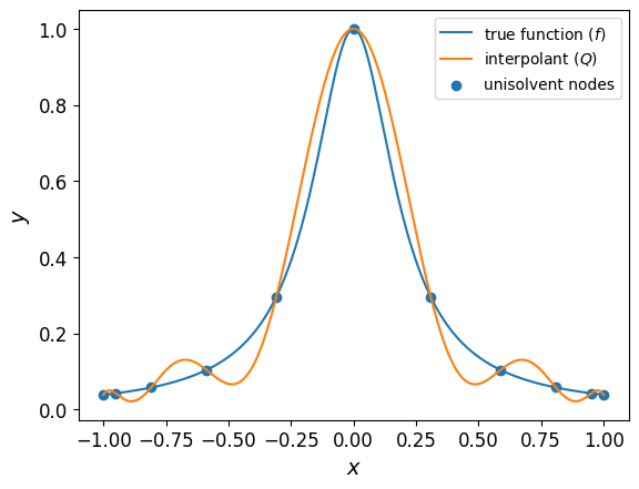
The plot also shows the location of the unisolvent nodes and their corresponding function values confirming that the polynomial passes through the unisolvent nodes.
Assess the accuracy of interpolating polynomial#
As shown in the plot above, the chosen polynomial degree is not accurate enough to approximate the true function.
The infinity norm provides a measure of the greatest error of the interpolant over the whole domain. The norm is defined as:
The infinity norm of \(Q\) can be approximated using the \(1'000\) testing points created above:
np.max(np.abs(yy_test - yy_poly))
np.float64(0.1321948529511282)
indicating that the interpolating polynomial of degree \(10\) is insufficient to accurately approximate the Runge function.
The interpolate() function#
As an alternative to constructing an interpolating polynomial from scratch using the steps outlined above, you can use the interpolate() function. The function allows you to specify:
the function to interpolate
the number of dimensions
the degree of polynomial interpolant
All in a single function call. The function returns a callable object that you can use to evaluate the (underlying) interpolating polynomial at a set of query points.
To create an interpolant using the interpolate() function with the same structure as before, use the following command:
q = mp.interpolate(fun, spatial_dimension=1, poly_degree=10)
The resulting interpolant can be evaluated at a set of query points:
q(xx_test)[:5]
array([0.03846154, 0.04058527, 0.04244967, 0.0440694 , 0.0454586 ])
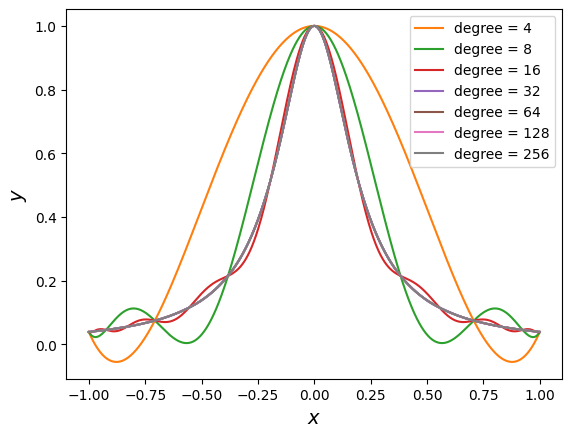
With this shortcut in hand, let’s investigate the convergence behavior of interpolating polynomials with increasing polynomial degrees.
poly_degrees = [4, 8, 16, 32, 64, 128, 256]
yy_poly = np.empty((len(xx_test), len(poly_degrees)))
for i, n in enumerate(poly_degrees):
    fx_interp = mp.interpolate(fun, spatial_dimension=1, poly_degree=n)
    yy_poly[:, i] = fx_interp(xx_test)
The interpolants of increasing degrees are shown below:
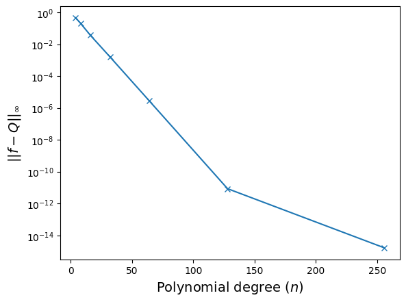
The convergence of the error is shown below:
errors = np.max(np.abs(yy_test[:, np.newaxis] - yy_poly), axis=0)
The absolute error of the degree 256 polynomials in the domain is shown below:
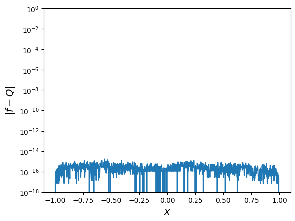
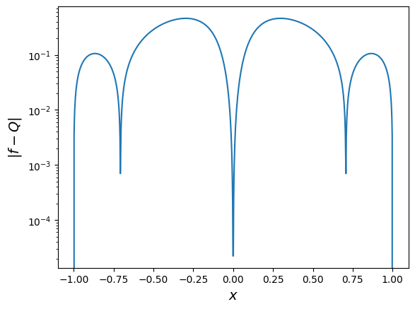
The seemingly random behavior of the (very small) absolute error indicates that machine precision has been reached. For comparison, the absolute error of the degree \(4\) polynomial is shown below:
plt.plot(xx_test, np.abs(yy_test - yy_poly[:, 0]))
plt.ylabel(r"$| f - Q |$", fontsize=14)
plt.xlabel("$x$", fontsize=14)
plt.yscale("log");
From interpolant to polynomial#
The callable produced by interpolate() is an instance of Interpolant; it is not a Minterpy polynomial per se.
There are, however, convenient methods to represent the interpolant as one of the Minterpy polynomial types. These methods are summarized in the table below.
Method |
Return the interpolant as a polynomial in the… |
|---|---|
These polynomial bases are covered in more detail in Polynomial Bases and Transformations in-depth tutorial.
For now, to obtain the lastly created interpolating polynomial in the Newton basis, call:
fx_interp.to_newton()
<minterpy.polynomials.newton_polynomial.NewtonPolynomial at 0x7f1be5c0e650>
Summary#
Congratulations on completing the first in-depth tutorial of Minterpy!
In this tutorial, you’ve learned how to create an interpolating polynomial from scratch in Minterpy to approximate a given function and evaluate it at a set of query points. Specifically, you covered:
Defining a multi-index set: Establishing the structure of the polynomial.
Constructing an interpolation grid: Creating the grid points (unisolvent nodes) for interpolation.
Evaluating the given function on the grid points: Computing function values at the nodes.
Constructing a polynomial in the Lagrange basis: Creating an interpolating polynomial in the Lagrange basis with the function values as the coefficients.
Transforming the polynomial into the Newton basis: Changing the basis from the Lagrange basis to the Newton basis for more evaluation and further manipulation.
You’ve also explored the interpolate() function, which simplifies the process of creating an interpolant.
Finally, you’ve learned how to assess the accuracy of an interpolating polynomial as an approximation of the given function and how to investigate its empirical convergence by adjusting the polynomial degree.
As its name implies, Minterpy is designed for multivariate polynomial interpolation. The process for constructing these polynomials follows similar steps to those described here.
In the next tutorial, you’ll learn how to create multivariate polynomials to interpolate multidimensional functions using Minterpy.