Quick Start Guide to Function Approximations with Minterpy

Welcome to the Quickstart Guide to Minterpy!

If you’re reading this, chances are you want to create an interpolant that approximates a function, possibly across multiple dimensions. This guide provides a quick walkthrough on how to achieve this using Minterpy.

How to import Minterpy

After installing installing Minterpy, you can import it as follows:

import minterpy as mp

The shorthand mp is the convention we, the developer team, like to use. You’re free to choose any shorthand you prefer, but we find mp to be both short and recognizable (similar to np for NumPy and pd for pandas).

While you’re at it, you will also need to import NumPy and Matplotlib to follow along with this guide.

import numpy as np
import matplotlib.pyplot as plt

One-dimensional function

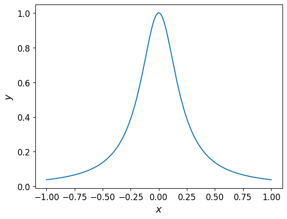
Let’s start with interpolating the following one-dimensional function:

\[ f(x) = \frac{1}{1 + 25 \, x^2}, \]

defined on \(x \in [-1, 1]\).

You can define the function above using lambda function:

fun_1d = lambda xx: 1 / (1 + 25 * xx**2)

When plotted, the function looks like this:

Show code cell source

Hide code cell source

xx_1d = np.linspace(-1, 1, 1000)
yy_1d = fun_1d(xx_1d)

plt.plot(xx_1d, yy_1d)
plt.xlabel("$x$", fontsize=14)
plt.ylabel("$y$", fontsize=14)
plt.tick_params(axis='both', which='major', labelsize=12);

One-dimensional interpolant

To create an interpolant in Minterpy, use the interpolate() function. It takes three arguments in order: the function to interpolate, the spatial dimension, and the polynomial degree.

The function must be a callable that accepts a two-dimensional array of shape (N, m) where m is the number of dimensions and returns a one-dimensional array of length N. The lambda function you defined above already satisfies this.

The spatial dimension is \(1\) since \(f\) takes a single input variable. Minterpy cannot infer this automatically, so you must specify it explicitly.

For the polynomial degree, higher degrees give better approximations at the cost of more function evaluations. As a best practice, always verify the accuracy of the interpolant after construction.

For instance, let’s say you choose a polynomial degree of \(8\):

interp_1d = mp.interpolate(fun_1d, spatial_dimension=1, poly_degree=8)
interp_1d

Interpolant()

Congratulations on creating your first interpolant in Minterpy!

Having obtained an interpolant, you can evaluate it at a set of query points:

xx_test_1d = np.linspace(-1, 1, 1000)  # 1000 query points
interp_1d(xx_test_1d)[:10]  # Show the first 10

array([0.03846154, 0.03614297, 0.03402996, 0.03211545, 0.03039255,
       0.02885446, 0.02749454, 0.0263063 , 0.02528334, 0.02441941])

The plot of the interpolant is shown below along with the original function:

Show code cell source

Hide code cell source

plt.plot(xx_1d, fun_1d(xx_1d), label="original")
plt.plot(xx_1d, interp_1d(xx_1d), label="interpolant")
plt.xlabel("$x$", fontsize=14)
plt.ylabel("$y$", fontsize=14)
plt.tick_params(axis='both', which='major', labelsize=12)
plt.legend(fontsize=14);

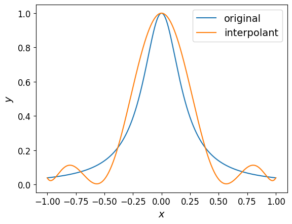
However, the interpolant doesn’t quite match the function as closely as we’d like.

Assessing 1D interpolant accuracy

Looking at the plot above, you might conclude that the interpolant is not accurate enough. But relying on a plot alone is not always possible, especially in higher dimensions.

The infinity norm provides a quantitative measure of the greatest (worst-case) error over the entire domain of the function:

\[ \lVert f - Q \rVert_\infty = \sup_{-1 \leq x \leq 1} \lvert f(x) - Q(x) \rvert \]

where \(Q\) is the Minterpy interpolant and \(\sup\) denotes the supremum, i.e., the least upper bound of the error across all points in the domain.

You can estimate the infinity norm based on a fine grid of test points, say \(1'000\) points:

np.max(np.abs(fun_1d(xx_test_1d) - interp_1d(xx_test_1d)))

np.float64(0.20467466589680205)

Whether that’s acceptable depends on your application. But for now, let’s agree that the current norm is far from numerically converged.

To have a more accurate interpolant, increase the polynomial degree, say to \(128\):

interp_1d_128 = mp.interpolate(fun_1d, spatial_dimension=1, poly_degree=128)

The plot of the interpolant is shown below.

Show code cell source

Hide code cell source

plt.plot(xx_1d, fun_1d(xx_1d), label="original")
plt.plot(xx_1d, interp_1d(xx_1d), label="interpolant (deg=8)")
plt.plot(xx_1d, interp_1d_128(xx_1d), label="interpolant (deg=128)")
plt.xlabel("$x$", fontsize=14)
plt.ylabel("$y$", fontsize=14)
plt.tick_params(axis='both', which='major', labelsize=12)
plt.legend(fontsize=14);

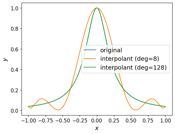
Looking at the graph, it’s hard to see any difference between the interpolant of degree \(64\) and the original function.

Looking at the infinity norm:

Show code cell source

Hide code cell source

np.max(np.abs(fun_1d(xx_test_1d) - interp_1d_128(xx_test_1d)))

np.float64(8.653744387743245e-12)

which is now closer to numerical convergence.

Two-dimensional function

Consider now a two-dimensional function taken from Cheng and Sandu (2010)[1]:

\[ f(x_1, x_2) = \cos{(x_1 + x_2)} \, e^{x_1 \, x_2}, \]

where \(x_1, x_2 \in [0, 1]\).

Below is the code to define the function above in Python as a regular function:

def fun_2d(xx):
    return np.cos(np.sum(xx, axis=1)) * np.exp(np.prod(xx, axis=1))

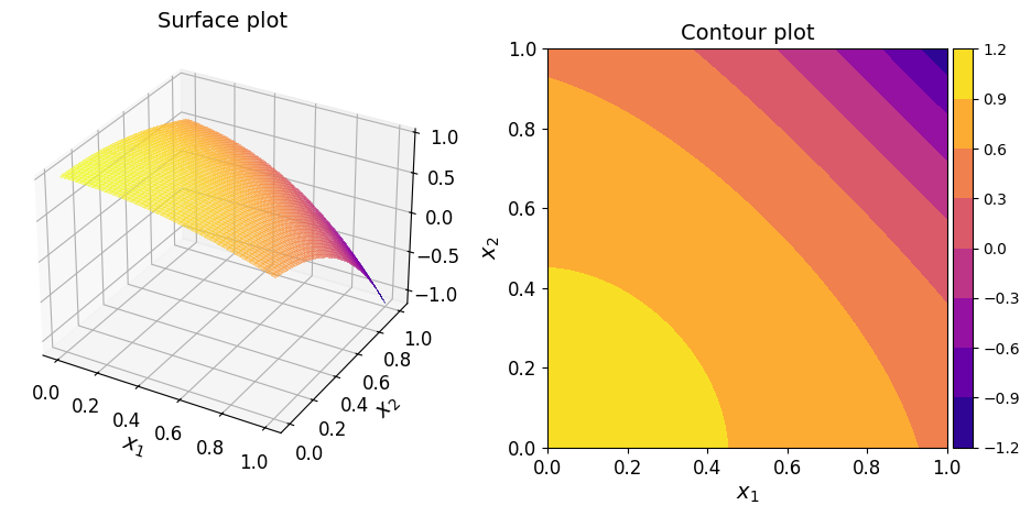
The surface and contour plots of the function are given below.

Show code cell source

Hide code cell source

from mpl_toolkits.axes_grid1 import make_axes_locatable

# --- Create 2D data
xx_1d = np.linspace(0, 1.0, 1000)[:, np.newaxis]
mesh_2d = np.meshgrid(xx_1d, xx_1d)
xx_2d = np.array(mesh_2d).T.reshape(-1, 2)
yy_2d = fun_2d(xx_2d)

# --- Create two-dimensional plots
fig = plt.figure(figsize=(10, 5))

# Surface
axs_1 = plt.subplot(121, projection='3d')
axs_1.plot_surface(
    mesh_2d[0],
    mesh_2d[1],
    yy_2d.reshape(1000,1000).T,
    linewidth=0,
    cmap="plasma",
    antialiased=False,
    alpha=0.5
)
axs_1.set_xlabel("$x_1$", fontsize=14)
axs_1.set_ylabel("$x_2$", fontsize=14)
axs_1.set_title("Surface plot", fontsize=14)
axs_1.tick_params(axis='both', which='major', labelsize=12)

# Contour
axs_2 = plt.subplot(122)
cf = axs_2.contourf(
    mesh_2d[0], mesh_2d[1], yy_2d.reshape(1000, 1000).T, cmap="plasma"
)
axs_2.set_xlabel("$x_1$", fontsize=14)
axs_2.set_ylabel("$x_2$", fontsize=14)
axs_2.set_title("Contour plot", fontsize=14)
divider = make_axes_locatable(axs_2)
cax = divider.append_axes('right', size='5%', pad=0.05)
fig.colorbar(cf, cax=cax, orientation='vertical')
axs_2.axis('scaled')
axs_2.tick_params(axis='both', which='major', labelsize=12)

fig.tight_layout(pad=3.0)

Two-dimensional interpolant

interpolate() can also handle two-dimensional functions. A few things to keep in mind when moving to two dimensions:

Function to interpolate. The callable requirement is the same as before. The only difference is that the input array now has two columns, one per spatial dimension.

Spatial dimension. Set spatial_dimension to \(2\) as Minterpy cannot infer this automatically.

Domain bounds. Since \(f\) is defined on \([0, 1]^2\) rather than the default \([-1, 1]^2\), you must specify the domain bounds explicitly via the bounds argument. The bounds are specified for every dimension. For the current example, bounds=[[0, 1], [0, 1]].

\(l_p\)-degree. For functions in more than one dimension, you can also specify the lp_degree argument, which controls the underlying multi-index set of exponents. Different values affect the structure and accuracy of the interpolant. See the relevant section for details. If not specified, it defaults to \(2.0\).

To create a two-dimensional interpolant with a polynomial degree of \(16\), use the following command:

interp_2d = mp.interpolate(
    fun_2d,
    spatial_dimension=2,
    poly_degree=16,
    bounds=[[0, 1], [0,1]],
)

The surface and contour plots of the interpolant are shown below.

Show code cell source

Hide code cell source

from mpl_toolkits.axes_grid1 import make_axes_locatable

# --- Create 2D data
xx_1d = np.linspace(0.0, 1.0, 500)[:, np.newaxis]
mesh_2d = np.meshgrid(xx_1d, xx_1d)
xx_2d = np.array(mesh_2d).T.reshape(-1, 2)
yy_2d = interp_2d(xx_2d)

# --- Create two-dimensional plots
fig = plt.figure(figsize=(10, 5))

# Surface
axs_1 = plt.subplot(121, projection='3d')
axs_1.plot_surface(
    mesh_2d[0],
    mesh_2d[1],
    yy_2d.reshape(500, 500).T,
    linewidth=0,
    cmap="plasma",
    antialiased=False,
    alpha=0.5
)
axs_1.set_xlabel("$x_1$", fontsize=14)
axs_1.set_ylabel("$x_2$", fontsize=14)
axs_1.set_title("Surface plot", fontsize=14)
axs_1.tick_params(axis='both', which='major', labelsize=12)

# Contour
axs_2 = plt.subplot(122)
cf = axs_2.contourf(
    mesh_2d[0], mesh_2d[1], yy_2d.reshape(500, 500).T, cmap="plasma"
)
axs_2.set_xlabel("$x_1$", fontsize=14)
axs_2.set_ylabel("$x_2$", fontsize=14)
axs_2.set_title("Contour plot", fontsize=14)
divider = make_axes_locatable(axs_2)
cax = divider.append_axes('right', size='5%', pad=0.05)
fig.colorbar(cf, cax=cax, orientation='vertical')
axs_2.axis('scaled')
axs_2.tick_params(axis='both', which='major', labelsize=12)

fig.tight_layout(pad=3.0)

Assessing 2D interpolant accuracy

Just by looking at the plot, it’s though to say for sure if the interpolant is accurate enough. But it does seem to capture the overall shape of the function pretty well.

As explained previously, you can use the infinity norm to quantify the accuracy of the interpolant. To estimate it using, say, \(100'000\) random points in \([0, 1]^2\):

rng = np.random.default_rng(194)
xx_test_2d = rng.random((100000, 2))
np.max(np.abs(fun_2d(xx_test_2d) - interp_2d(xx_test_2d)))

np.float64(2.55351295663786e-15)

The choice of polynomial degree seems to be already results in a highly accurate interpolant.

Four-dimensional function

So far, you’ve seen how to interpolate 1D and 2D functions. But what about functions with even more dimensions?

Consider now the \(m\)-dimensional Runge function:

\[ f(\boldsymbol{x}) = \frac{1}{1 + \lVert \boldsymbol{x} \rVert_2^2}, \]

defined on \([-1, 1]^m.\)

The function can be computed for any dimension, but for this tutorial we set \(m = 4\). The dimension is high enough to make direct visualization impractical.

Note

The classic Runge function has a factor of \(25\) instead of \(1.0\) which makes the classic function sharper and thus harder to interpolate accurately.

To define the function above as a lambda function:

fun_md = lambda xx: 1 / (1 + 1.0 * np.sum(xx**2, axis=1))

Four-dimensional interpolant

The \(m\)-dimensional Runge function is chosen to show that interpolate() works the same way regardless of dimension. The callable requirement is the same as before; the input array now has four columns, one per spatial dimension.

Since \(f\) is defined on \([-1, 1]^4\), which is the default domain, you don’t need to specify the bounds argument explicitly.

Just like with 2D functions, you can also tweak the \(l_p\)-degree of the underlying multi-index set for higher-dimensional functions (\(m > 1\)). While this is optional and can affect the accuracy of the interpolant, the default value of \(2.0\) is a reasonable choice.

To create a 4D interpolant with a polynomial degree of \(16\), use the following command:

interp_4d = mp.interpolate(fun_md, spatial_dimension=4, poly_degree=16)

Assessing 4D interpolant accuracy

As before, you can use the infinity norm to gauge the accuracy of the interpolant. To estimate it using \(10'000\) random points in \([-1, 1]^4\), you can use the following code:

xx_test_4d = -1 + rng.random((10000, 4))
np.max(np.abs(fun_md(xx_test_4d) - interp_4d(xx_test_4d)))

np.float64(1.7148324011895255e-05)

For an additional cost, you can improve the accuracy of the interpolant by increasing the polynomial degree.

Summary

That’s it for the Quickstart Guide!

You’ve seen how to interpolate functions in one, two, and four dimensions using interpolate() and how to specify custom domain bounds.

---

Minterpy offers much more than what’s covered here. If you’d like to explore further, we’ve prepared a series of tutorials covering the more advanced features of Minterpy.

---

[1]

Haiyan Cheng and Adrian Sandu. Collocation least-squares polynomial chaos method. In Proceedings of the 2010 Spring Simulation Multiconference, SpringSim ‘10, 1–6. Society for Computer Simulation International, 2010. doi:10.1145/1878537.1878621.