Polynomial Regression with Minterpy#

The polynomials you’ve worked with in these tutorials are designed to approximate functions of interest by using values at specific, strategically chosen points that form unisolvent nodes.

However, you may face a situation where you cannot choose the evaluation points freely: function values are available only at arbitrary, scattered points across the domain. Despite this limitation, it is possible to derive a polynomial that best fits the scattered data using the least squares method.

In this tutorial, you’ll learn how to perform polynomial regression in Minterpy to construct a polynomial that best approximates the available data.

As usual, before you begin, you’ll need to import the necessary packages to follow along with this guide.

import matplotlib.pyplot as plt
import minterpy as mp
import numpy as np
import warnings

warnings.filterwarnings("ignore", category=UserWarning)

Motivating problem#

Consider the following two-dimensional function:

\[ f(\boldsymbol{x}) = \frac{1}{\sqrt{2}} \left( f_1(x_1) f_1(x_2) + f_2(x_1) f_2(x_2) \right), \]

where

\[\begin{split} \begin{aligned} f_1(x) & = \frac{1}{\pi^{1/4}} e^{-x^2/2} \\ f_2(x) & = \frac{2 x}{\sqrt{\pi}} f_1(x), \end{aligned} \end{split}\]

and \(\boldsymbol{x} = (x_1, x_2) \in [0, 1.5]^2\).

First, define the above functions in Python:

def fun_1(x):
    return 1 / np.pi**(1 / 4) * np.exp(-0.5 * x**2)

def fun_2(x):
    return fun_1(x) * (2 * x) / np.sqrt(np.pi)

def fun(xx):
    return 1 / np.sqrt(2) * fun_1(xx[:, 0]) * fun_1(xx[:, 1]) + fun_2(xx[:, 0]) * fun_2(xx[:, 1])

Then, generate the dataset randomly, say with \(100\) points:

rng = np.random.default_rng(9271)
xx_train = 1.5 * rng.random((100, 2))
yy_train = fun(xx_train)

The plots of the function along with the given dataset are shown below.

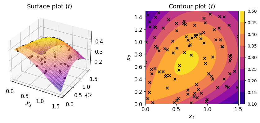
../_images/031f2b083fdd7691b7152dbc528502b84cbd315c32033871a809d1b1e06b417a.png

Given a dataset of pairs \(\{ (\boldsymbol{x}^{(i)}, y^{(i)}) \}_{i = 1}^N\), your task is to construct a polynomial that approximates the function. In a typical regression setting, unlike here, the underlying function is unknown and you only have access to the dataset.

Polynomial regression#

In polynomial regression, a linear system of equations is constructed as follows:

\[ \boldsymbol{R} \, \boldsymbol{c} = \boldsymbol{y}, \]

where \(\boldsymbol{R}\), \(\boldsymbol{c}\), \(\boldsymbol{y}\) are the regression matrix, the vector of polynomial coefficients, and the vector of output data, respectively.

Each column of the regression matrix \(\boldsymbol{R}\) is obtained by evaluating each of the monomials of the chosen polynomial basis at all input data points.

The goal of polynomial regression is to estimate \(\boldsymbol{c}\) given \(\{ (\boldsymbol{x}^{(i)}, y^{(i)}) \}_{i = 1}^N\).

Define a multi-index set#

Start with defining the underlying multi-index set.

For instance, you may define a multi-index set of polynomial degree \(8\) and \(l_p\)-degree \(2.0\):

mi = mp.MultiIndexSet.from_degree(2, 8, 2.0)

Make sure that the size of the multi-index set is no larger than the available data points.

len(mi)

Define a domain#

Because the domain of the function is not the default domain of \([-1, 1]^m\), you need to specify a domain.

You can use the uniform() factory method to create a uniform rectangular domain for a given spatial dimension and bounds:

dom = mp.Domain.uniform(2, 0, 1.5)

Create an ordinary regression polynomial#

The OrdinaryRegression class is the interface between the polynomials that you’ve seen before and a regression polynomial.

To create an instance of OrdinaryRegression, pass the multi-index set to the default constructor:

reg_poly = mp.OrdinaryRegression(mi, domain=dom)

Fit the regression polynomial#

So far, the coefficients of your regression polynomial remain unknown:

reg_poly.coeffs is None

True

The polynomial coefficients are obtained by solving the following least-squares problem:

\[ \hat{\boldsymbol{c}} = \underset{\boldsymbol{c}}{\mathrm{arg min}} \lVert \boldsymbol{R} \boldsymbol{c} - \boldsymbol{y} \rVert_2^2 \]

where \(\lVert \cdot \rVert_2^2\) denotes the square of the Euclidean norm.

By default, the regression matrix \(\boldsymbol{R}\) is constructed by evaluating the monomials of the Lagrange basis (defined with respect to the Leja-ordered Chebyshev-Lobatto points) at the input data points. Consequently, the estimated coefficients \(\hat{\boldsymbol{c}}\) are the coefficients of the polynomial in the Lagrange basis.

You can use the method fit() to solve the above problem on your regression polynomial. It requires the input points and the corresponding output values:

reg_poly.fit(xx_train, yy_train)

Note that the call to fit() alters the instance in-place; once the call is concluded, the coefficients are available:

reg_poly.coeffs[:10]  # the first 10

array([0.1294195 , 0.39896156, 0.30113665, 0.17577316, 0.38943229,
       0.35839612, 0.23301724, 0.14081214, 0.39829943, 0.21241999])

Evaluate the regression polynomial#

Once fitted, you can evaluate the regression polynomial at a set of query points in the user-defined domain. For instance, the line below evaluates the regression polynomial on three points in:

reg_poly(
    np.array([
        [0., 1.],
        [0., 0.],
        [0., 0.5],
    ])
)

array([0.2419698 , 0.39896156, 0.35206169])

Verify the fitted polynomial#

You can also check several measures that indicate the quality of the fitted polynomial by calling the show() on your regression polynomial:

reg_poly.show()

Ordinary Polynomial Regression
------------------------------
Spatial dimension: 2
Poly. degree     : 8
Lp-degree        : 2.0
Origin poly.     : <class 'minterpy.polynomials.lagrange_polynomial.LagrangePolynomial'>
Error                     Absolute     Relative
L-inf Regression Fit   5.04134e-07  7.60417e-06
L2 Regression Fit      2.34905e-14  5.34448e-12
LOO CV                 2.61940e-11  5.95956e-09

The three measures of fitting error are summarized in the table below.

Metric	Absolute error	Relative error (normalized by)
`L-inf`	\(\max_i \lvert y^{(i)} - \hat{f}(\boldsymbol{x}^{(i)}) \rvert\)	Standard deviation of \(\boldsymbol{y}\)
`L2`	\(\frac{1}{N}\sum_i ( y^{(i)} - \hat{f}(\boldsymbol{x}^{(i)}) )^2\)	Variance of \(\boldsymbol{y}\)
`LOO CV`	\(\frac{1}{N}\sum_i ( y^{(i)} - \hat{f}_{\setminus i}(\boldsymbol{x}^{(i)}) )^2\)	Variance of \(\boldsymbol{y}\)

Note that for L2 and LOO CV the errors are still squared.

These fitting error measures are solely based on the training dataset. You should view them critically; small values do not necessarily mean highly accurate regression polynomial as they tend to underestimate the generalization error (i.e., error based on the unseen data).

That being said, the LOO CV error is usually a more robust estimate of the generalization error than the other two: the L-inf error tends to be overly conservative, while the L2 error is directly minimized during fitting and therefore tends to underestimate the generalization error.

To estimate the generalization error in the L2 sense:

xx_test = 1.5 * rng.random((10000, 2))
yy_test = fun(xx_test)
print(np.mean((yy_test - reg_poly(xx_test))**2))

1.0605947423621413e-11

The plots below show the surface, contour, and the error plot for the regression polynomial.

Show code cell source

Hide code cell source

from mpl_toolkits.axes_grid1 import make_axes_locatable

# --- Create 2D data
xx_1d = np.linspace(0, 1.5, 500)[:, np.newaxis]
mesh_2d = np.meshgrid(xx_1d, xx_1d)
xx_2d = np.array(mesh_2d).T.reshape(-1, 2)
yy_fun_2d = fun(xx_2d)
yy_reg_2d = reg_poly(xx_2d)
yy_err_2d = np.abs(yy_fun_2d - yy_reg_2d)

# --- Create two-dimensional plots
fig = plt.figure(figsize=(15, 5))

# Surface
axs_1 = plt.subplot(131, projection='3d')
axs_1.plot_surface(
    mesh_2d[0],
    mesh_2d[1],
    yy_reg_2d.reshape(500, 500).T,
    linewidth=0,
    cmap="plasma",
    antialiased=False,
    alpha=0.4,
)
axs_1.scatter(
    xx_train[:, 0],
    xx_train[:, 1],
    yy_train,
    color="k",
    marker="x",
)
axs_1.set_xlabel("$x_1$", fontsize=14)
axs_1.set_ylabel("$x_2$", fontsize=14)
axs_1.set_title("Surface plot ($Q_f$)", fontsize=14)
axs_1.tick_params(axis='both', which='major', labelsize=12)

# Contour
axs_2 = plt.subplot(132)
cf = axs_2.contourf(
    mesh_2d[0], mesh_2d[1], yy_reg_2d.reshape(500, 500).T, cmap="plasma"
)
axs_2.scatter(xx_train[:, 0], xx_train[:, 1], color="k", marker="x")
axs_2.set_xlabel("$x_1$", fontsize=14)
axs_2.set_ylabel("$x_2$", fontsize=14)
axs_2.set_title("Contour plot ($Q_f$)", fontsize=14)
divider = make_axes_locatable(axs_2)
cax = divider.append_axes('right', size='5%', pad=0.05)
fig.colorbar(cf, cax=cax, orientation='vertical')
axs_2.axis('scaled')
axs_2.tick_params(axis='both', which='major', labelsize=12)

# Contour Eror
axs_3 = plt.subplot(133)
cf = axs_3.contourf(
    mesh_2d[0], mesh_2d[1], yy_err_2d.reshape(500, 500).T, cmap="plasma"
)
axs_3.scatter(xx_train[:, 0], xx_train[:, 1], color="k", marker="x")
axs_3.set_xlabel("$x_1$", fontsize=14)
axs_3.set_ylabel("$x_2$", fontsize=14)
axs_3.set_title("Error ($| f - Q_f |$)", fontsize=14)
divider = make_axes_locatable(axs_3)
cax = divider.append_axes('right', size='5%', pad=0.05)
fig.colorbar(cf, cax=cax, orientation='vertical')
axs_3.axis('scaled')
axs_3.tick_params(axis='both', which='major', labelsize=12)

fig.tight_layout()

../_images/c94836c5888fbf04122dcd36c26ec6f106f48f1672412d60d5951c43543fce83.png

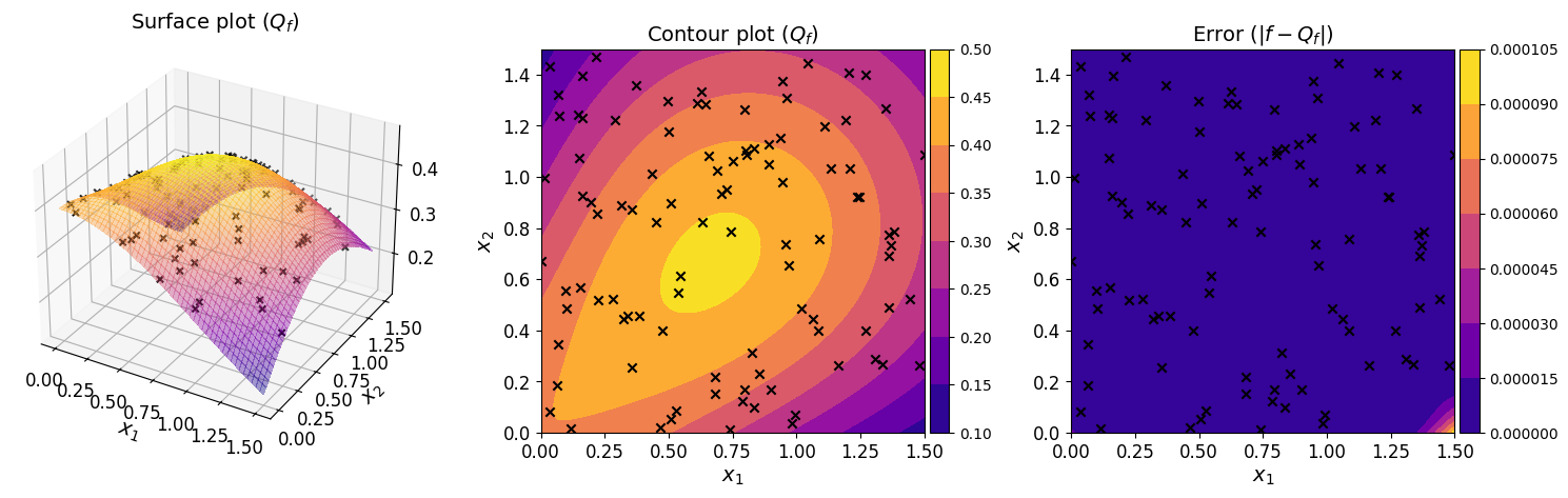
The plots show that the regression polynomial captures the overall behavior of the original function well, consistent with the small generalization error estimated above.

Accessing the fitted polynomial#

Once fitted, a regression polynomial is fully determined. In particular, the eval_poly property of the instance is a Minterpy polynomial you’re already familiar. You can carry out arithmetic an calculus operations on it.

reg_poly.eval_poly

<minterpy.polynomials.newton_polynomial.NewtonPolynomial at 0x7f447b744b20>

By default, the evaluation polynomial is a polynomial in the Newton basis.

Summary#

In this tutorial, you’ve learned how to perform polynomial regression using Minterpy. This is particularly useful when working with a dataset consisting of input–output pairs, especially when the underlying function is unknown or inaccessible.

Polynomial regression in Minterpy is available through the OrdinaryRegression class. To construct a regression polynomial for a given dataset:

Determine the structure of the underlying polynomial by specifying the multi-index set and user-defined domain
Create an instance of OrdinaryRegression based on the defined polynomial structure
Fit the instance with the given dataset using the fit() method
Verify the regression polynomial using the show() method

Once fitted, the resulting instance is callable, allowing you to evaluate it at any set of query points in the user-defined domain by passing these points directly to the instance.

Finally, you can access the underlying fitted polynomial via the eval_poly, which is a Minterpy polynomial that supports a variety of arithmetic and calculus operations on it, as covered in the previous tutorials.

Congratulations on completing this series of Minterpy in-depth tutorials!

You should now be familiar with the main features of Minterpy. We hope you find Minterpy valuable for your work!