Basic Arithmetic Operations with Polynomials

Once you’ve constructed a polynomial in Minterpy, you can do more than just evaluate it. This tutorial shows how to perform arithmetic operations with Minterpy polynomials. Specifically, you’ll learn that Minterpy polynomials are closed under the following operations:

• Adding or subtracting one polynomial to/from another

• Adding or subtracting a real scalar number to/from a polynomial

• Multiplying a polynomial by another polynomial

• Multiplying a polynomial by a real scalar number

• Raising a polynomial to a non-negative integer power

In other words, each of these operations produces another Minterpy polynomial in the same basis.

To keep things simple, the examples in this tutorial use one-dimensional polynomials, but the principles apply to Minterpy polynomials of any dimension.

Before you start, make sure to import the necessary packages to follow along with this guide.

import minterpy as mp
import numpy as np
import matplotlib.pyplot as plt

Motivating functions

Consider the following two one-dimensional functions.

The first is the sine function:

\[ f_1(x) = \sin{(5 \pi x)}, x \in [-1, 1]. \]

You can define the above function as a lambda function in Python:

fun_1 = lambda xx: np.sin(5 * np.pi * xx)

Following the examples given in the previous guide, you can construct an interpolating polynomial of the function above as follows:

# Multi-index set of polynomial degree 30
mi_1 = mp.MultiIndexSet.from_degree(1, 30)
# Interpolation grid
grd_1 = mp.Grid(mi_1)
# Coefficients of the Lagrange polynomial
coeffs_1 = grd_1(fun_1)
# Lagrange polynomial given grid and coefficients
lag_poly_1 = mp.LagrangePolynomial.from_grid(grd_1, coeffs_1)
# Transformation to the Newton basis
poly_1 = mp.LagrangeToNewton(lag_poly_1)()                 

You can check the infinity norm of the polynomial to decide if the approximation is good enough.

xx_test = -1 + 2 * np.random.rand(10000)
yy_test_1 = fun_1(xx_test)
yy_poly_1 = poly_1(xx_test)
print(np.max(np.abs(yy_poly_1 - yy_test_1)))

3.9777197002877074e-07

Note

The choice of polynomial degree above is just an example; in practice, you will have to decide what level of accuracy is sufficient for your specific use case. Also, keep in mind that infinity norm is just one way to measure accuracy; other common metrics, like mean-squared error, are also widely used.

The second is the exponential function:

\[ f_2(x) = 2.0 \, e^{-2.5 (x + 1)}, x \in [-1, 1]. \]

As before, you can define the function as a lambda function:

fun_2 = lambda xx: 2.0 * np.exp(-2.5 * (xx + 1))

and then the interpolating polynomial:

# Multi-index set of polynomial degree 15
mi_2 = mp.MultiIndexSet.from_degree(1, 15)
# Interpolation grid
grd_2 = mp.Grid(mi_2)
# Coefficients of the Lagrange polynomial
coeffs_2 = grd_2(fun_2)
# Lagrange polynomial given grid and coefficients
lag_poly_2 = mp.LagrangePolynomial.from_grid(grd_2, coeffs_2)
# Transformation to the Newton basis
poly_2 = mp.LagrangeToNewton(lag_poly_2)()

Finally, check the approximation accuracy via the infinity norm:

yy_test_2 = fun_2(xx_test)
yy_poly_2 = poly_2(xx_test)
print(np.max(np.abs(yy_poly_2 - yy_test_2)))

1.226574397605873e-12

The plots of both interpolating polynomials are shown below.

Show code cell source

Hide code cell source

xx_plot = np.linspace(-1, 1, 500)

fig, axs = plt.subplots(nrows=1, ncols=2, figsize=(10, 4))

axs[0].plot(xx_plot, fun_1(xx_plot), label="true function")
axs[0].plot(xx_plot, poly_1(xx_plot), label="polynomial ($Q$)")
axs[0].scatter(grd_1.unisolvent_nodes[:, 0], coeffs_1)
axs[0].set_xlabel("$x$", fontsize=14);
axs[0].set_ylabel("$f_1(x)$", fontsize=14);
axs[0].set_title("Sine", fontsize=16);
axs[0].tick_params(axis='both', which='major', labelsize=12)


axs[1].plot(xx_plot, fun_2(xx_plot), label="true function ($f$)")
axs[1].plot(xx_plot, poly_2(xx_plot), label="polynomial ($Q$)")
axs[1].scatter(grd_2.unisolvent_nodes[:, 0], coeffs_2, label="interpolating nodes")
axs[1].set_xlabel("$x$", fontsize=14);
axs[1].set_ylabel("$f_2(x)$", fontsize=14);
axs[1].set_title("Exponential", fontsize=16)
axs[1].tick_params(axis='both', which='major', labelsize=12)
axs[1].legend(fontsize=14)

fig.tight_layout()

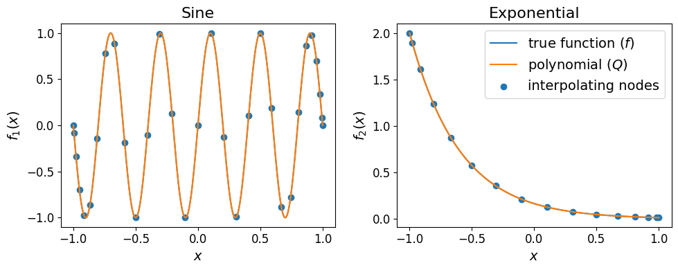
The plots show that there are no notable differences between the two true functions and their corresponding interpolating polynomials

---

Now that you have the two interpolating polynomials, you can start doing arithmetic operations with them.

Addition and subtraction

Minterpy polynomials support addition and subtraction with real scalar numbers; the result is another polynomial in the same basis.

For instance:

poly_scalar_add = poly_1 + 5
poly_scalar_add

<minterpy.polynomials.newton_polynomial.NewtonPolynomial at 0x7f881a6bf880>

or:

poly_scalar_sub = poly_1 - 5
poly_scalar_sub

<minterpy.polynomials.newton_polynomial.NewtonPolynomial at 0x7f881aa1c220>

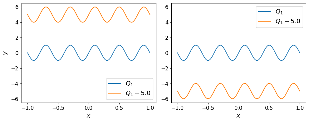
Adding (resp. subtracting) a real scalar number uniformly shifts the polynomial up (resp. down):

Show code cell source

Hide code cell source

# Use the same points for plotting

fig, axs = plt.subplots(nrows=1, ncols=2, figsize=(10, 4))

axs[0].plot(xx_plot, poly_1(xx_plot), label="$Q_1$")
axs[0].plot(xx_plot, poly_scalar_add(xx_plot), label="$Q_1 + 5.0$")
axs[0].set_xlabel("$x$", fontsize=14)
axs[0].set_ylabel("$y$", fontsize=14)
axs[0].tick_params(axis='both', which='major', labelsize=12)
axs[0].legend(fontsize=14, loc="lower right")
axs[0].set_ylim([-6.5, 6.5])

axs[1].plot(xx_plot, poly_1(xx_plot), label="$Q_1$")
axs[1].plot(xx_plot, poly_scalar_sub(xx_plot), label="$Q_1 - 5.0$")
axs[1].set_xlabel("$x$", fontsize=14);
axs[1].tick_params(axis='both', which='major', labelsize=12)
axs[1].legend(fontsize=14, loc="upper right")
axs[1].set_ylim([-6.5, 6.5])

fig.tight_layout();

Polynomials may also be added or subtracted from each other; the result is once again another polynomial.

For instance, \(Q_{\mathrm{sum}} = Q_1 + Q_2\):

poly_sum = poly_1 + poly_2
poly_sum

<minterpy.polynomials.newton_polynomial.NewtonPolynomial at 0x7f88186cabf0>

or \(Q_{\mathrm{diff}} = Q_1 - Q_2\):

poly_diff = poly_1 - poly_2
poly_diff

<minterpy.polynomials.newton_polynomial.NewtonPolynomial at 0x7f881850acb0>

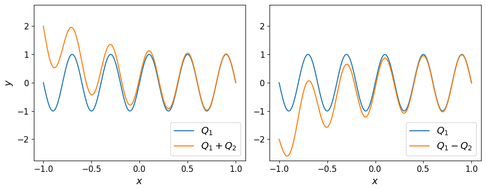
The plots of the two polynomials are shown below.

Show code cell source

Hide code cell source

# Use the same points for plotting

fig, axs = plt.subplots(nrows=1, ncols=2, figsize=(10, 4))

axs[0].plot(xx_plot, poly_1(xx_plot), label="$Q_1$")
axs[0].plot(xx_plot, poly_sum(xx_plot), label="$Q_1 + Q_2$")
axs[0].set_xlabel("$x$", fontsize=14)
axs[0].set_ylabel("$y$", fontsize=14)
axs[0].tick_params(axis='both', which='major', labelsize=12)
axs[0].legend(fontsize=14, loc="lower right")
axs[0].set_ylim([-2.75, 2.75])

axs[1].plot(xx_plot, poly_1(xx_plot), label="$Q_1$")
axs[1].plot(xx_plot, poly_diff(xx_plot), label="$Q_1 - Q_2$")
axs[1].set_xlabel("$x$", fontsize=14);
axs[1].tick_params(axis='both', which='major', labelsize=12)
axs[1].legend(fontsize=14, loc="lower right")
axs[1].set_ylim([-2.75, 2.75])

fig.tight_layout();

Note

Addition and subtraction between two polynomials requires both to be defined on the same domain. If the domains differ, Minterpy raises a DomainMismatchError. When no domain is specified, polynomials are defined on the default internal reference domain \([-1, 1]^m\). This, therefore, is not a concern in the examples above.

Multiplication

Minterpy polynomials may also be multiplied by a real scalar number; the operation returns another polynomial.

Consider \(5 \times Q_2\):

poly_scalar_mul = 5.0 * poly_2
poly_scalar_mul

<minterpy.polynomials.newton_polynomial.NewtonPolynomial at 0x7f88186b8fd0>

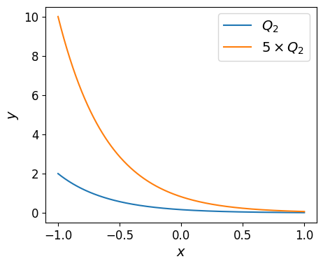
Scalar multiplication uniformly scales the polynomial across its domain as shown in the plot below.

Show code cell source

Hide code cell source

fig, ax = plt.subplots(nrows=1, ncols=1, figsize=(5, 4))

ax.plot(xx_plot, poly_2(xx_plot), label="$Q_2$")
ax.plot(xx_plot, poly_scalar_mul(xx_plot), label="$5 \\times Q_2$")
ax.set_xlabel("$x$", fontsize=14)
ax.set_ylabel("$y$", fontsize=14)
ax.tick_params(axis='both', which='major', labelsize=12)
ax.legend(fontsize=14);

Furthermore, a multiplication between Minterpy polynomials is a valid operation that returns a polynomial.

For instance, \(Q_{\mathrm{prod}} = Q_1 \times Q_2\):

poly_prod = poly_1 * poly_2
poly_prod

<minterpy.polynomials.newton_polynomial.NewtonPolynomial at 0x7f881aa1ccd0>

The plot of the product polynomial is shown below:

Show code cell source

Hide code cell source

fig, axs = plt.subplots(nrows=1, ncols=3, figsize=(12, 4))

axs[0].plot(xx_plot, poly_1(xx_plot), label="$Q_1$")
axs[0].set_xlabel("$x$", fontsize=14)
axs[0].set_ylabel("$y$", fontsize=14)
axs[0].tick_params(axis='both', which='major', labelsize=12)
axs[0].legend(fontsize=14, loc="upper right")
axs[0].set_ylim([-2.0, 2.25])

axs[1].plot(xx_plot, poly_2(xx_plot), label="$Q_2$")
axs[1].set_xlabel("$x$", fontsize=14);
axs[1].tick_params(axis='both', which='major', labelsize=12)
axs[1].legend(fontsize=14, loc="upper right")
axs[1].set_ylim([-2.0, 2.25])

axs[2].plot(xx_plot, poly_prod(xx_plot), label="$Q_1 \\times Q_2$")
axs[2].set_xlabel("$x$", fontsize=14)
axs[2].tick_params(axis='both', which='major', labelsize=12)
axs[2].legend(fontsize=14, loc="upper right")
axs[2].set_ylim([-2.0, 2.25])

fig.tight_layout();

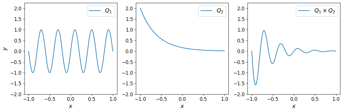
The product polynomial is an exponentially decaying sine function. This is a consequence of multiplying a sine by a decaying exponential.

Division

Minterpy polynomials may be divided by a real scalar number; this operation returns another polynomial.

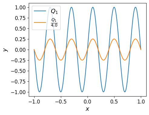
For instance, \(Q_1 / 4.0\):

poly_scalar_div = poly_1 / 4.0
poly_scalar_div

<minterpy.polynomials.newton_polynomial.NewtonPolynomial at 0x7f881a76a2f0>

Division by a real scalar number uniformly scales the polynomial across its domain as shown in the plot below.

Show code cell source

Hide code cell source

fig, ax = plt.subplots(nrows=1, ncols=1, figsize=(5, 4))

ax.plot(xx_plot, poly_1(xx_plot), label="$Q_1$")
ax.plot(xx_plot, poly_scalar_div(xx_plot), label="$\\frac{Q_1}{4.0}$")
ax.set_xlabel("$x$", fontsize=14)
ax.set_ylabel("$y$", fontsize=14)
ax.tick_params(axis='both', which='major', labelsize=12)
ax.legend(fontsize=14);

Minterpy, however, does not support polynomial-polynomial division. Specifically the expression

\[ Q_3 = \frac{Q_1}{Q_2} \]

is a rational function which, in general, cannot be represented as a polynomial.

Note

That being said, you can still evaluate the expression above at a given set of query points where \(Q_2(x) \neq 0\).

Exponentiation

Finally, Minterpy polynomials may also be exponentiated by a non-negative integer. As with all the other arithmetic operations above, polynomial exponentiation returns another polynomial.

For instance, \(Q_1^2\):

poly_exp = poly_1**2
poly_exp

<minterpy.polynomials.newton_polynomial.NewtonPolynomial at 0x7f881a9bd0c0>

Show code cell source

Hide code cell source

fig, ax = plt.subplots(nrows=1, ncols=1, figsize=(5, 4))

ax.plot(xx_plot, poly_1(xx_plot), label="$Q_1$")
ax.plot(xx_plot, poly_exp(xx_plot), label="$Q_1^2$")
ax.set_xlabel("$x$", fontsize=14)
ax.set_ylabel("$y$", fontsize=14)
ax.tick_params(axis='both', which='major', labelsize=12)
ax.legend(fontsize=14);

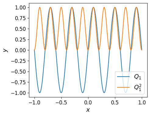
Raising a polynomial to a non-negative integer power is equivalent to repeatedly multiplying the polynomial by itself.

For instance, \(Q_2^2 = Q_2 \times Q_2\):

poly_2**2 == poly_2 * poly_2

True

or \(Q_2^3 = Q_2 \times Q_2 \times Q_2\):

poly_2**3 == poly_2 * poly_2 * poly_2

True

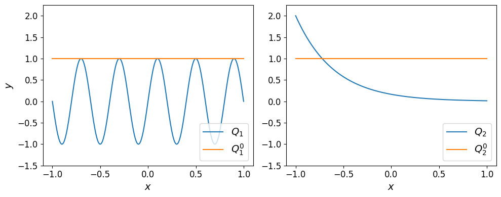
Finally, raising a polynomial to the power of \(0\) results in a constant polynomial with a value of \(1.0\).

poly_1_exp_0 = poly_1**0
poly_2_exp_0 = poly_2**0

Show code cell source

Hide code cell source

fig, axs = plt.subplots(nrows=1, ncols=2, figsize=(10, 4))

axs[0].plot(xx_plot, poly_1(xx_plot), label="$Q_1$")
axs[0].plot(xx_plot, poly_1_exp_0(xx_plot), label="$Q_1^0$")
axs[0].set_xlabel("$x$", fontsize=14)
axs[0].set_ylabel("$y$", fontsize=14)
axs[0].tick_params(axis='both', which='major', labelsize=12)
axs[0].legend(fontsize=14, loc="lower right")
axs[0].set_ylim([-1.5, 2.25])

axs[1].plot(xx_plot, poly_2(xx_plot), label="$Q_2$")
axs[1].plot(xx_plot, poly_2_exp_0(xx_plot), label="$Q_2^0$")
axs[1].set_xlabel("$x$", fontsize=14);
axs[1].tick_params(axis='both', which='major', labelsize=12)
axs[1].legend(fontsize=14, loc="lower right")
axs[1].set_ylim([-1.5, 2.25])

fig.tight_layout();

Warning

Minterpy polynomials do not support exponentiation by another polynomial, a negative number, or a non-integer value. If you attempt to perform such an operation, an exception will be raised.

Summary

In this in-depth tutorial, you’ve learned about the basic arithmetic operations involving Minterpy polynomials. Minterpy polynomials are closed under the following arithmetic operations, meaning that the result of performing these operations is always another Minterpy polynomial:

• Polynomial-scalar addition and subtraction

• Polynomial-polynomial addition and subtraction

• Polynomial-scalar multiplication

• Polynomial-polynomial multiplication

• Polynomial-scalar division

• Polynomial exponentiation by a non-negative integer

Throughout the tutorial, one-dimensional polynomials were used for illustration, but the same principles apply to Minterpy polynomials of any dimension.

Minterpy currently does not support:

• Polynomial-polynomial division (i.e., forming rational functions)

• Polynomial exponentiation by another polynomial or by a real scalar (including negative integers and non-integer numbers)

Additionally, polynomial-polynomial operations require both polynomials to share the same domain; otherwise a DomainMismatchError is raised.

---

In the next tutorial, you will explore additional features of Minterpy, including basic calculus operations such as differentiation and integration.