
Interpolation at Unisolvent Nodes#
The construction of a multi-dimensional interpolating polynomial relies on a set of carefully selected points in the domain and a chosen polynomial basis. The points must be selected such that the polynomial of a given degree can be uniquely determined, that is, the points are unisolvent.
This page introduces the required points for this construction and the selected polynomial basis for interpolation.
Generating points#
The generating points of degree \(n_j\) are selected by choosing arbitrary set of points \(P_j \subseteq [-1,1]\) with \(|P_j| = n_j + 1 \in \mathbb{N}\) points for each dimension \(m \in \mathbb{N}\), such that for a fixed multi-index set \(A \subseteq \mathbb{N}\), it holds that \(n_j \geq \max \{\alpha_j : \alpha \in A\}\).
Chebyshev-Lobatto points
When \(A = A_{m, n, p}\) is defined by a multi-index set of specified polynomial degree \(n\) and math:l_p-degree \(p\), the points are typically chosen to tbe the Chebyshev-Lobatto points:
Other prominent choices of generating points are the Gauss-Legendre points, Chebyshev points of first & second kind, equidistant points, see for example[1][2][3].
Matrix of generating points
The generating points are stored as a matrix where each column represents the chosen set of points for a particular dimension. Specifically, the matrix is constructed by stacking the chosen set of points for each dimension column-wise. That is,
Leja ordering
The choice of the ordering of the generating points is crucial for the stability of the interpolating polynomial. We assume that the generating points \(P_j\) are Leja-ordered[4], which means that they satisfy the following conditions:
The Leja ordering of the generating points not only ensures the numerical stability of the Newton interpolation, but also results in unisolvent nodes forming a (sparse, non-tensorial) grid with high approximation power.
Unisolvent nodes#
For a multi-index set \(A \subseteq \mathbb{N}^m\) and chosen generating points \(\mathrm{GP} = \oplus_{j = 1}^m P_j\) the unisolvent nodes \(P_A\) are given as the sub-grid
In addition to the possibly different choices of the \(P_j\) in each dimension, the impact of different orderings can be observed in the example below (Fig. 3).
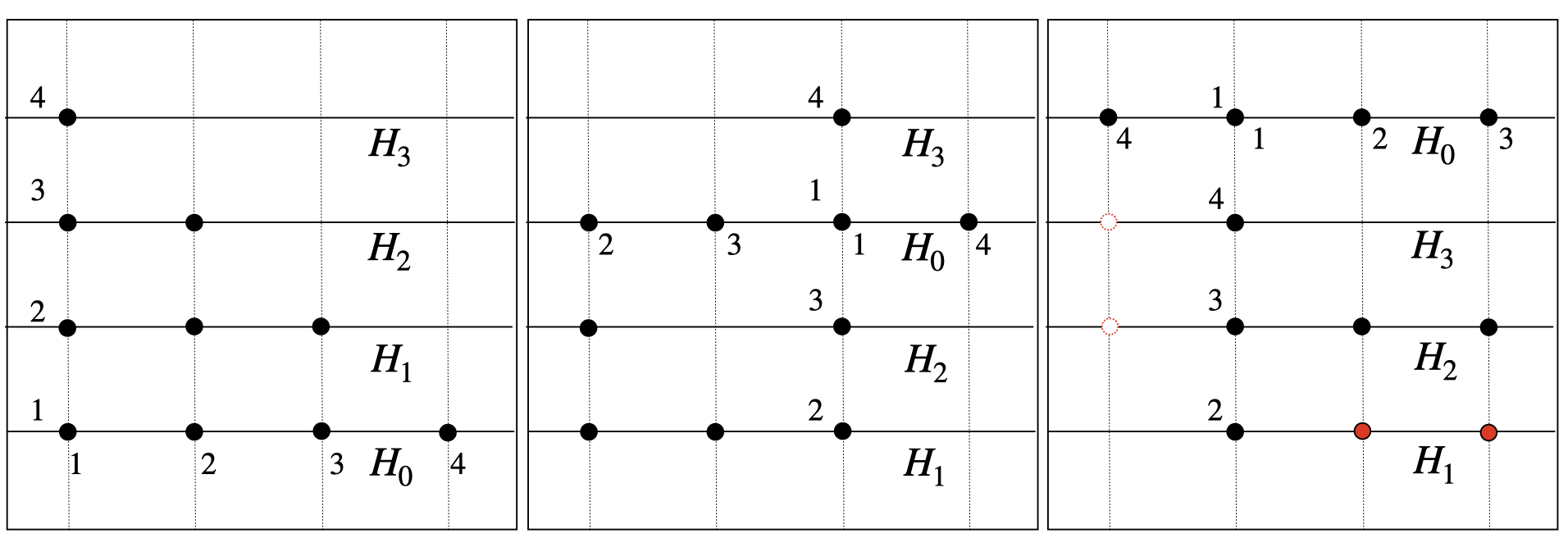
Fig. 3 Unisolvent nodes for \(A= A_{2,3,1}\) (left, middle) and \(A_{2,3,2}\) (right). Orderings in \(x,y\)–directions are indicated by numbers and non-tensorial nodes \(p=(p_x,p_y) \in P_A\) in red with missing symmetric blank counter parts \((p_y,p_x)\not \in P_A\).#
In the figure, the sets \(P_j\) differ only in their orderings, as indicated by the enumerations along the dimensions (\(x, y\)). The resulting unisolvent nodes may form non-tensorial or non-symmetric grids, where nodes exist with \(p=(p_x, p_y) \in P_A\), but \((p_y, p_x) \not \in P_A\).
Examples of unisolvent nodes in two dimensions and three dimensions for the default choice of the Leja-ordered Chebyshev-Lobatto nodes are visualized below.
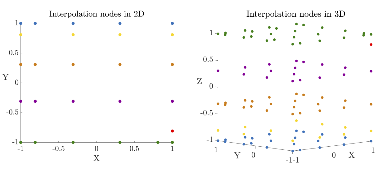
Fig. 4 Leja ordered Chebyshev-Lobatto nodes for Euclidian \(l_2\)-degree \(n = 5\).#
From a general perspective, a more detailed discussion of their construction and resulting properties is available[5]. Crucially, for downward-closed multi-index sets \(A \subseteq \mathbb{N}^m\), the interpolating polynomial \(Q_{f,A}\) is uniquely determined in the polynomial space
spanned by all canonical basis polynomials.
Lagrange interpolation#
Given:
a multi-index set \(A \subseteq \mathbb{N}^m\) for \(m \in \mathbb{N}\),
unisolvent nodes \(P_A \subseteq \Omega = [-1,1]^m\), and
a function \(f: \Omega\longrightarrow \mathbb{R}\),
the uniquely determined interpolating polynomial in the Lagrange basis \(Q_{f,A}\) of \(f\) is given by
where \(L_\alpha\) denote the Lagrange basis polynomial that satisfy \(L_{\alpha}(p_\beta) = \delta_{\alpha,\beta}\) with \(\delta_{\cdot,\cdot}\) denoting the Kronecker delta.
In fact, deriving the interpolating polynomial in the Lagrange basis \(Q_{f,A}\) of a function \(f\) is straightforward and can be obtained with linear \(\mathcal{O}(|A|)\) storage amount and runtime complexity provided that the unisolvent nodes \(P_A\) are given.
However, interpolation polynomial in the Lagrange basis is rather a theoretical construct in Minterpy because the computational scheme for evaluating the polynomial at a query point is non-trivial. In particular, the closed-form formula for the Lagrange monomials is difficult to derive for non-tensorial multi-index sets.
Newton interpolation#
As an alternative to the interpolating polynomial in the Lagrange basis, the same polynomial in the Newton basis is given by
where \(A \subseteq \mathbb{N}^m\) is a set of multi-indices, \(N_\alpha\) are the Newton basis polynomial with respect to the generating points \(\mathrm{GP}\), and \(c_{\mathrm{nwt}, \alpha}\) are the corresponding Newton coefficients.
The coefficients \(c_{\mathrm{nwt}, \alpha}\) can be derived by the multi-dimensional divided difference scheme (DDS) for a given generating points \(\mathrm{GP}\). The scheme requires quadratic \(\mathcal{O}(|A|^2)\) runtime complexity and linear \(\mathcal{O}(|A|)\) storage.
References