Multidimensional Divided Difference Scheme (DDS)

Splitting Theorems

The Multivariate DDS is based on two general splitting Theorems[1] that can be stated in a simplified version as:

Theorem 1 (Splitting of unisolvent nodes) Let \(A \subseteq \mathbb{N}^m\) be a downward closed multi-index set, \(\Pi_A =\left<x^\alpha = x_1^{\alpha_1}\cdots x_m^{\alpha_m} : \alpha \in A\right>\) be the polynomial space spanned by all monomials induced by \(A\), \(H = \{(x_1,\dots,x_m) \in \mathbb{R}^m : x_j = y\}, y \in [-1,1]\) for some \(1\leq j \leq m\) be a hyperplane parallel to the coordinate axis, \(Q_H= (x_j - q_j) \in \Pi_A\) and \(P \subseteq \mathbb{N}^m\) be a set of nodes such that:

\(i)\) There is no polynomial \(Q \in \Pi_A\) being constant in normal direction to \(H\), i.e., \(\partial_{x_j}Q(x) =0\), and \(Q\) vanishes identically on \(P \cap H\), i.e., \(Q(p) =0\,, \forall \,p \in P \cap H\).

\(ii)\) There is no polynomial \(Q \in \Pi_A\) with \(Q_H\cdot Q \in \Pi_A\) and \(Q\) vanishes identically on \(P \setminus H\), i.e, \(Q(p) =0\,, \forall \, p \in P \setminus H\).

Then, the nodes \(P\) are unisolvent with respect to \(\Pi_A\), i.e, the interpolant \(Q_{f,A}(p) = f(p) \,, \forall \, p \in P\) of any function \(f : \mathbb{R}^m \longrightarrow \mathbb{R}\) is uniquely determined in \(\Pi_A\).

Below, we show examples of unisolvent nodes in 2D for \(A= A_{2,3,1}\), generated by recursively applying Theorem 1. The three panels show examples for three different choices of the, in this case 1D, hyperplanes \(H_0,\ldots ,H_3\) (solid lines). In the left panel, the hyperplanes are chosen arbitrarily. This starts by first choosing a hyperplane (line) \(H_0\) and \(n+1=4\) unisolvent nodes on \(H_0\). Then choose \(H_1 \not = H_0\) and 3 unisolvent nodes on \(H_1 \setminus H_0\), and recursively continue until choosing 1 unisolvent node on \(H_3\setminus (H_0 \cup H_1 \cup H_2)\). When choosing the hyperplanes parallel to each other, as shown in the middle panel, this construction results in an irregular grid. Quantizing the distance between hyperplanes as well as between nodes on them further leads to non-tensorial grids, as shown in the right panel.

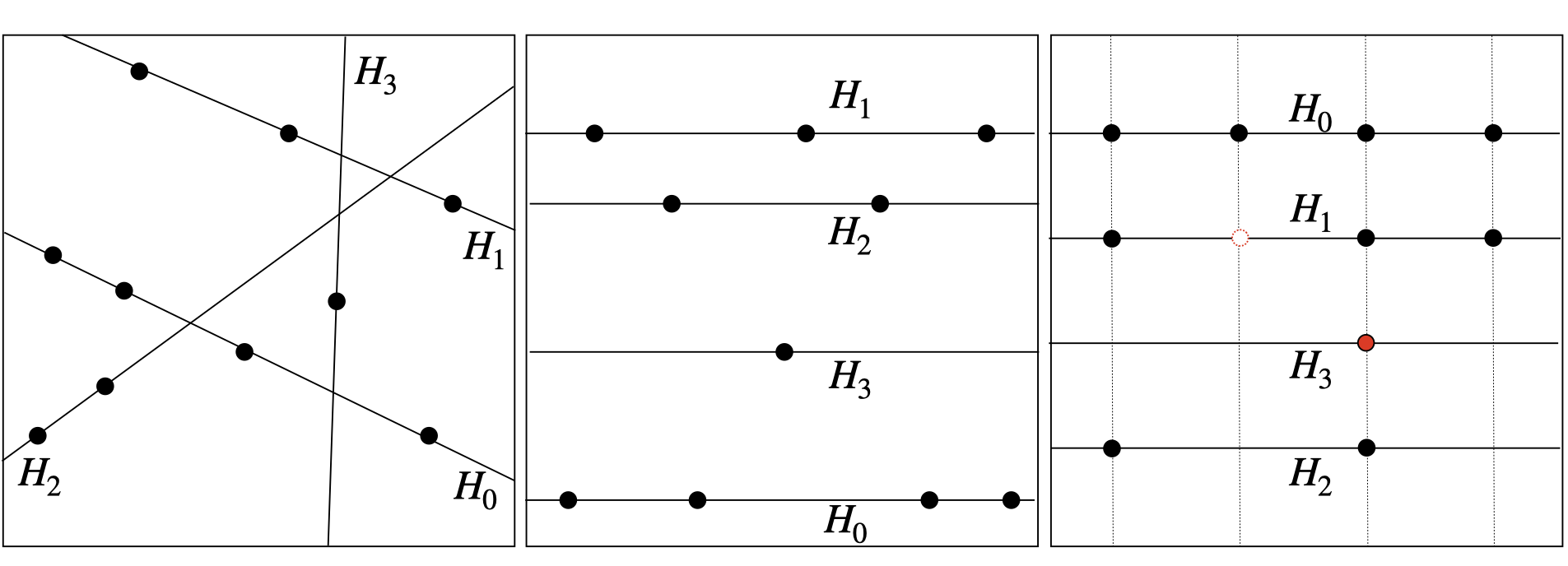
Fig. 5 Examples of unisolvent nodes.

Theorem 2 (Splitting of the interpolant) Let the assumptions of Theorem 1 be satisfied. Let in addition

\(i)\) \(Q_1 \in \Pi_{A}\) be a polynomial being constant in normal direction to \(H\) interpolating \(f\) in \(P\cap H\), i.e, \(Q_{f,A}(p) = f(p) \,, \forall \, p \in P\cap H\)

\(ii)\) \(Q_2 \in \Pi_{A}\) be a polynomial with \(Q_H\cdot Q_2 \in \Pi_A\) interpolating \(f_1:=(f -Q_1)/Q_H\) in \(P\setminus H\), i.e,

(7)\[Q_{f,A}(p) = f_1(p) =(f(p) - Q_1(p))/Q_H(p) \,, \quad \forall \, p \in P\setminus H.\]

Then the unique interpolant \(Q_{f,A}(p)\in \Pi_{A}\) is given by

\[Q_{f,A} = Q_1 + Q_H \cdot Q_2 \,.\]

In principle, the multivariate DDS is given by recursively applying Theorems 1 & 2. The generalised divided difference scheme given by recursively choosing suitable hyper(sub)planes \(H_{0}, H_{1,0}, H_{0,1}, \ldots\) and nodes \(P=P_0 =P_{1,0}\cup P_{0,1}, \ldots\) accordingly to Theorem 1 and applying the splitting Theorem 2 to the separated polynomials \(Q_1,Q_2,Q_{1,0},Q_{2,0},Q_{1,1},Q_{2,1},\ldots\) as visulaised below.

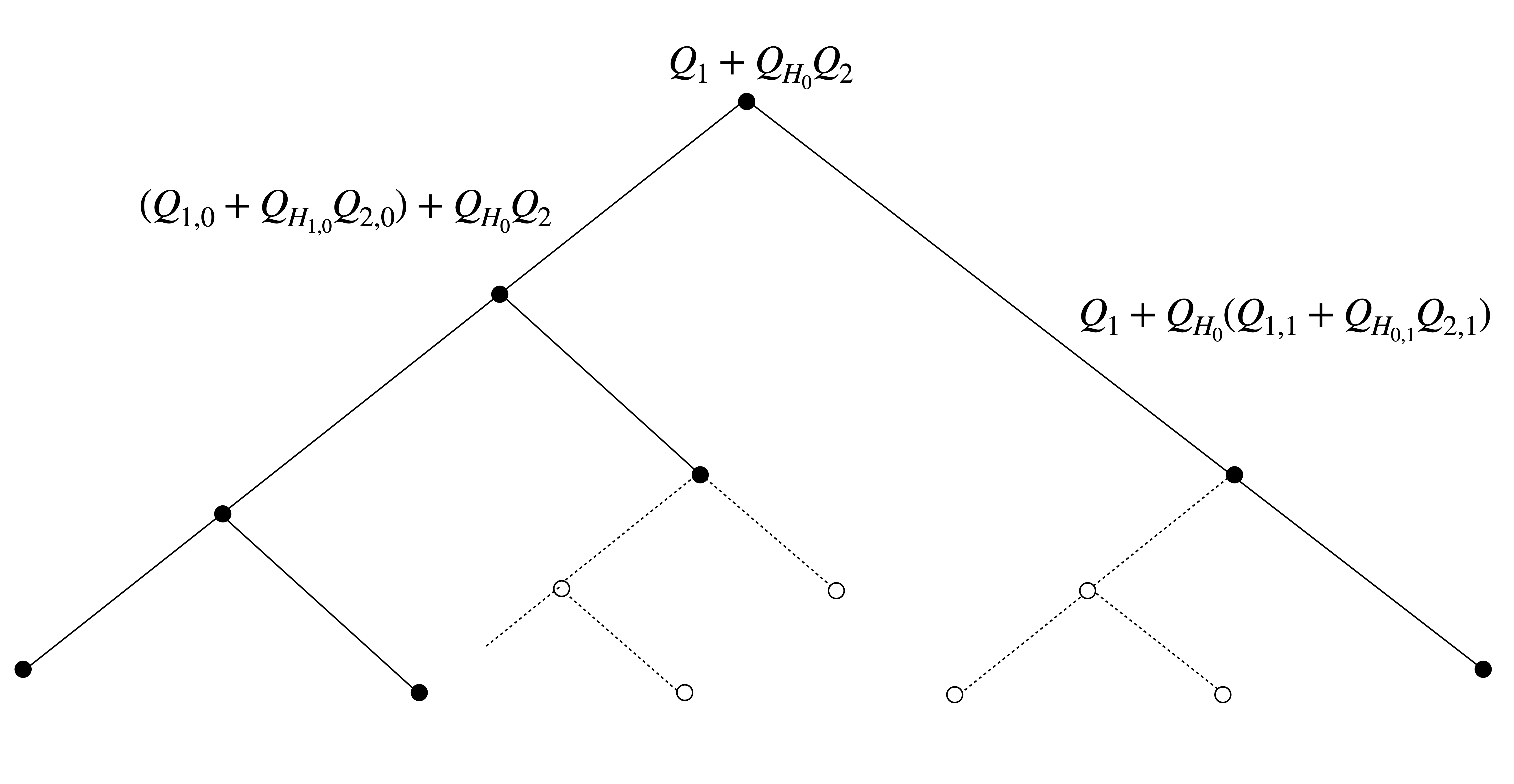
Fig. 6 The general multivariate Divided difference Scheme.

While in general the DDS requires \(\mathcal{O}(|A|^3)\) runtime complexity, faster implementations can be realised whenever the hyperplanes are chosen to be parallel and thereby the resulting unisolvent nodes are given as a sub-grid.

1D Divided Difference Scheme

We recapture the classic 1D DDS being the algorithmic solution of 1D Newton interpolation, see e.g.[2][3]. Given \(n+1\) distinct nodes \(p_0,\ldots, p_n\in [-1,1]\) and a function \(f : [-1,1] \longrightarrow \mathbb{R}\) one recursively defines

\[[p_i]f = f(p_i) \,,\quad [p_i,\dots,p_j]f:= \frac{[p_{i+1},\dots,p_j]f -[p_i,\dots,p_{j-1}]f}{p_j-p_i}\,, \,\, j> i\,.\]

The resulting Newton coefficients, are set as \(c_i:= [p_0,\dots,p_i]f\), and uniquely determine the interpolant \(Q_{f,A}\), \(A= A_{1,n,1}= \{0,\ldots,n\}\) in Newton form, i.e.,

(8)\[Q_{f,A}(x) = \sum_{i=0}^n c_i N_{i}(x)\,, \quad N_i(x) = \prod_{j=0}^{i-1}(x-p_j)\,.\]

The recursive 1D DDS is thereby classically visualised as follows:

\[\begin{split}\begin{matrix} [p_0]f \\ & \searrow \\{} [p_1]f & \rightarrow & [p_0,p_1]f \\ & \searrow & & \searrow \\{} [p_2]f & \rightarrow & [p_1,p_2]f & \rightarrow & [p_0,p_1,p_2]f \\{} \vdots & \vdots & \vdots & \vdots & \vdots &\ddots \\{} & \searrow & & \searrow & & & \searrow \\{} [p_{n}]f & \rightarrow & [p_{n-1},p_{n}]f & \rightarrow & [p_{n-2},p_{n-1},p_{n}]f & \cdots & \rightarrow & [p_0\ldots p_{n}]f \\ \end{matrix}\end{split}\]

Alternatively, by observing that a hyperplane \(H\subseteq \mathbb{R}\) in 1D is given by a point \(p \in \mathbb{R}\) and a polynomial \(Q\) in zero variables is a real number one can re-interpretate the nodes \(p_i\subseteq \mathbb{R}\) as hyperplanes \(H_i\subseteq \mathbb{R}\), \(0 \leq i \leq n\) and the values \([p_i,\ldots,p_j]f \in \mathbb{R}\) as polynomials and recursively apply the splitting Theorems 1 & 2 in order to observe the following tree decompostion of the problem.

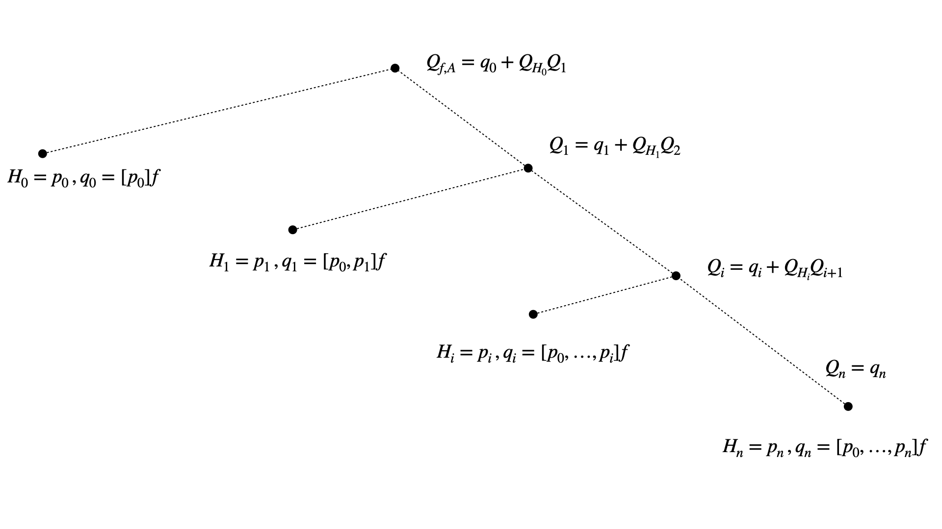
Fig. 7 The 1D DDS from the perspective of Theorems 1 & 2.

Thus, by using the Newton polynomials from Eq. (8) and observing that in this special 1D case Eq. (7) yields \(f_1(p) = [p_0,p_1]f\) we derive

\[\begin{split}Q_{f,A} &= q_0 + Q_{H_0}\Big(q_1 + \ldots + Q_{H_{i-1}}\big(q_i + \ldots + Q_{H_{n-1}}q_n \big) \ldots \Big)\\ &= \sum_{i=0}^n [p_0,\ldots,p_i]f \, \prod_{j=0}^{i-1}Q_{H_i}\\ &= \sum_{i=0}^n c_i \prod_{j=0}^{i-1}(x- p_j)\\ &= \sum_{i=0}^n c_i N_i(x)\,.\end{split}\]

In light of this perspective, we can visualise the the recursion of the 1D-DDS in a dependency graph resting on the underlying tree structure as given below:

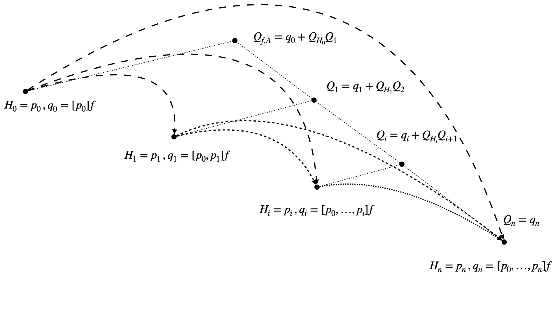
Fig. 8 Visulaisation of the dependencies of the leaf nodes accordingly to the 1D-DDS.

In order to generalise the tree decomposition of the Newton interpolation to multi-dimensions, we introduce the Multi-index tree allowing to decode the dependencies given by recursively applying Theorems 1 & 2 for the multi-dimensional case in a compactified way.

Multi-index tree

The multi-index tree provides the data structure that is needed to generalise the classic 1D Divided Difference Scheme of degree \(n \in \mathbb{N}\) to downward closed multi-index sets \(A \subseteq \mathbb{N}^m\), e.g. \(A =A_{m,n,p}\).

Here, we give an example for dimension \(m=3\) degree \(n=3\) with respect to Euclidian \(l_p\)-degree \(p=2\). As visualised below the multi-index set \(A_{3,3,2}\) is splitted into subsets that yield the corresponding interpolation sub problems.

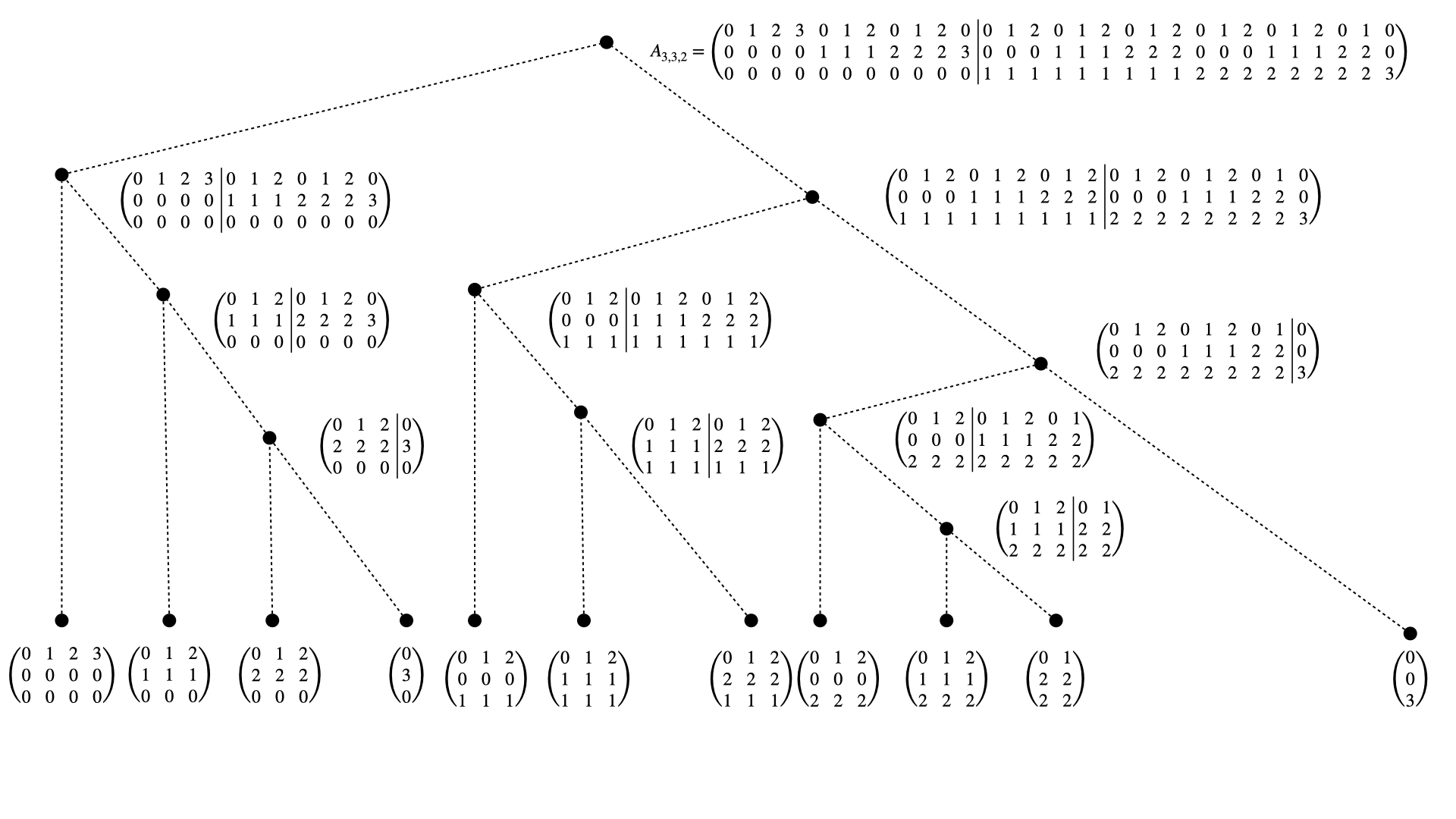
Fig. 9 The tree structure of the splitting of the multi-indices \(\alpha \in A_{3,3,2}\).

As one can observe, the splitting separates multi-indices \(\alpha, \beta \in A\) whenever they differ in the higher dimensional entries \(\alpha_j \not = \beta_j\,, 1 \leq j \leq m\) depending on the considered dimension \(j\). In other words: The splitting assigns multi-indices to the same sub-tree whenever all higher dimensional entries coincide \(\alpha_i = \beta_i\,, \forall \, i \geq j\). The split positions and subtree sizes are thereby stored when constucting the multi-index-tree.

Splitting of the unisolvent nodes

Each of the leafs of the multi-index tree induces an unisolvent interpolation node and the splitting reflects the parallel 1 & 2 dimensional hyper-sub-planes(lines) \(H \subseteq \mathbb{R}^m\) to which the nodes belong.

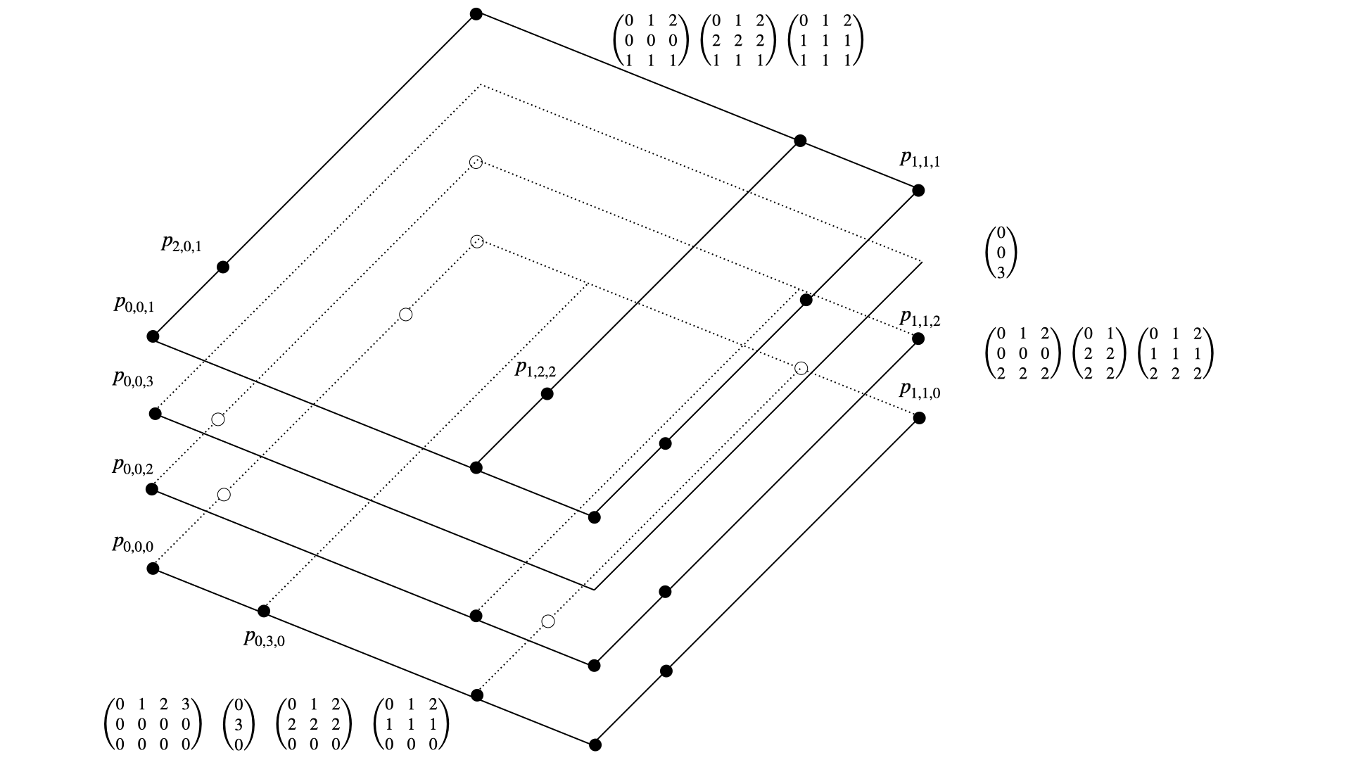
Fig. 10 The splitting of the multi-indicies is reflected in the geometric separation of the corresponding unisolvent nodes \(P_A=\left\{p_\alpha = (p_{\alpha_1,1},p_{\alpha_2,2},p_{\alpha_3,3}) : \alpha \in A \right\}\).

Sub-tree recursion

Indeed the node distributions on each hyperplane \(H\) are subsetes of the projections of the prior (more occupied) plane. This fact is refleceted when fixing the highest dimension and treating the subtrees belonging to lower dimensional problems as nodes. The dependencies and recursion of the multivariate DDS with respect to that highest fixed dimensions result in the prior considered ones of the 1D-DDS as visualised below.

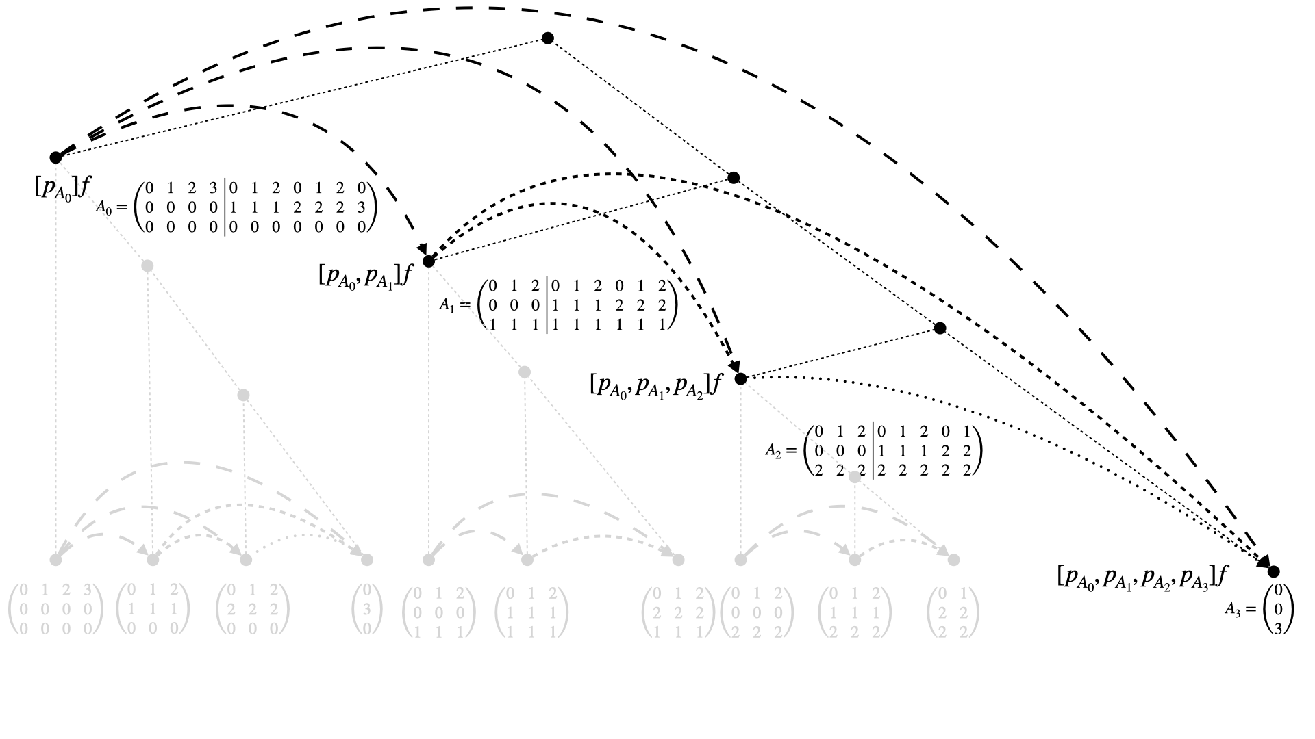
Fig. 11 First recursion step of the multivariate DDS (fixing the highest dimension).

The recursion step is thereby realised by using a precomputed mask that matches the nodes/multi-indicies of each sub-problem/hyperplane to the next one, accordingly. The recursion is analogously repeated for each subtree independently as sketched (in grey) above.

References

[1]

Michael Hecht, Krzysztof Gonciarz, Jannik Michelfeit, Vladimir Sivkin, and Ivo F Sbalzarini. Multivariate interpolation on unisolvent nodes–lifting the curse of dimensionality. arXiv preprint arXiv:2010.10824, 2020.

[2]

Josef Stoer and Roland Bulirsch. Introduction to numerical analysis. Volume 12. Springer Science & Business Media, 2002.

[3]

Walter Gautschi. Numerical analysis. Birkhäuser Boston, 2012. doi:10.1007/978-0-8176-8259-0.